Integrated Analysis of Post-Translational Modifications and Total Proteome: Methods for Distinguishing Abundance from Usage Changes

Witold Wolski

Antje Dittmann

Christian Panse

Laura Kunz

Jonas Grossmann

2025-07-15

Author	Affiliation(s)	Corresponding Author Email
Witold Wolski	FGCZ, SIB	witold.wolski@fgcz.uzh.ch
Antje Dittmann	FGCZ	antje.dittmann@fgcz.uzh.ch
Laura Kunz	FGCZ
Christian Panse	FGCZ, SIB
Jonas Grossmann	FGCZ, SIB	jonas.grossmann@fgcz.uzh.ch

• FGCZ - Functional Genomics Center Zurich, Winterthurerstrasse 190, CH-8057 Zurich,
• SIB - Swiss Institute of Bioinformatics, Winterthurerstrasse 190, CH-8057 Zurich

Abstract

Post-translational modifications (PTMs), particularly phosphorylation, regulate protein function at substoichiometric levels, making their quantitative analysis technically challenging. A critical limitation in PTM studies is distinguishing between changes in modification abundance due to altered protein expression versus genuine changes in modification stoichiometry (the fraction of protein molecules that are modified).

This chapter presents a comprehensive workflow integrating Tandem-Mass-Tag (TMT)-based quantitative proteomics with specialized computational analysis to distinguish differential PTM abundance (DPA) from differential PTM usage (DPU) using the prolfqua, prolfquapp, and prophosqua R packages. The workflow introduces a robust statistical framework for integrated PTM-protein analysis, comprehensive visualization tools including N-terminus to C-terminus (N-to-C) plots for protein-centric PTM mapping, and sequence motif analysis for kinase prediction.

This integrated approach enables researchers to identify actual signaling changes in PTM studies, prioritize functionally relevant modification sites, understand pathway-level regulation in disease contexts, and generate robust datasets suitable for publication in high-impact journals.

Key Words

Post-translational modifications, phosphoproteomics, TMT labeling, differential PTM abundance analysis, differential PTM usage analysis, mass spectrometry, data integration, kinase activity

Introduction

Biological Significance of Post-Translational Modifications

Protein phosphorylation is a reversible PTM that modulates a protein’s conformation, enzymatic activity, subcellular localization, or binding interactions. Because this modification can be reversed rapidly, it acts as a molecular switch in cellular signaling networks. As a result, cells respond to environmental cues without requiring new protein synthesis. Dysregulation of phosphorylation is implicated in cancer, neurodegeneration, and metabolic disorders [1]. Large-scale phosphoproteomic profiling by high-throughput mass spectrometry (MS) (e.g., TMT-based workflows) is therefore crucial for dissecting disease-associated signaling alterations and identifying candidate therapeutic targets.

Technical Challenges in PTM Analysis

The analysis of PTMs, such as phosphorylation, presents significant analytical challenges due to the low abundance of modified peptides. Typically, phosphorylated peptides represent less than 1–5% of the total peptide population [2]. Additionally, phosphopeptides generally exhibit poorer ionization efficiency in MS-based proteomics compared to non-modified peptides, further complicating their detection and quantification. This low abundance and challenging ionization behavior necessitate specialized experimental workflows and computational strategies to achieve accurate quantification [3].

A key analytical challenge is distinguishing genuine changes in PTM levels, due to altered kinase and phosphatase activity, from changes caused by altered protein abundance [4, 5]. Without proper correction, this confounding factor can lead researchers to misinterpret PTM data, incorrectly attributing higher phosphorylation signals solely to increased modification efficiency or pathway activation, rather than to elevated protein expression [6]. Controlling for this confounder is critical to discern rapid, signaling-driven phosphorylation events from slower, transcriptionally or translationally regulated changes in protein abundance.

Because phosphorylation is substoichiometric, only a small fraction of protein molecules carry the modification; therefore, enrichment is required to isolate phosphopeptides. Enrichment steps (such as Immobilized Metal Affinity Chromatography (IMAC) or Metal Oxide Affinity Chromatography (MOAC)) introduce additional sample handling and technical variability [6–8]. Therefore, each stage, from digestion to cleanup to MS acquisition, must be carefully optimized to improve reproducibility [9]. Effective experimental design combined with tailored normalization strategies is therefore essential to recover reliable, biologically meaningful PTM signals.

Isobaric TMT labeling enables multiplexed PTM analysis of up to 35 samples in a single run, reducing inter-sample variability and missing values to improve statistical power [10, 11]. Phosphopeptides are typically enriched by IMAC or Metal Oxide Affinity Chromatography (MOAC), which provide complementary selectivity and broaden coverage [12, 13]. Adding offline fractionation before liquid chromatography–tandem mass spectrometry (LC–MS/MS) further increases phosphosite depth and distributes peptide load, improving quantification consistency across fractions and conditions [14].

In TMT-based proteomics, a plex refers to the complete set of isobarically tagged samples analyzed together in a single LC–MS/MS run. When the total number of samples exceeds the available TMT channels, each plex should include at least one biological replicate from every experimental group and a common reference or pooled channel for normalization [15]. Replicates of the same group are then distributed across different plexes rather than clustered within a single run, preventing any group’s replicates from being confined to one batch. If all samples fit within the channel capacity of a single plex, these balancing measures are inherently satisfied in that run.

Computational Tools and Workflows

The computational landscape for quantitative protein PTM analysis has undergone significant evolution, with numerous specialized software platforms supporting bottom-up proteomics workflows. Following MS data acquisition, spectra undergo database searching to identify peptide sequences, which is subsequently followed by protein inference to determine protein identities based on these identified peptides. The ecosystem of PTM analysis includes several well-established data-dependent acquisition (DDA)-TMT compatible software suites, both free and commercial, such as Andromeda integrated within MaxQuant [16], Proteome Discoverer (Thermo Fisher Scientific), FragPipe [17], or PeptideShaker [18].

Among the analytical steps following peptide identification, PTM site localization scoring represents a particularly crucial computational challenge. Site localization determines the confidence with which a modification can be assigned to a specific amino acid residue within a peptide sequence. This process is especially challenging when peptides contain multiple potential modification sites, necessitating algorithms to evaluate the quality and specificity of site-determining fragment ions. Specialized tools have been developed explicitly for robust PTM site localization, including PTMProphet [19], PhosphoRS [20], and Ascore [21]. Accurate localization is essential, as incorrect site assignments can lead to biological misinterpretations, particularly in signaling pathway analyses and kinase-substrate predictions.

In DDA workflows, FragPipe [22] represents a widely adopted and integrated platform that comprehensively addresses PTM analysis, including site localization challenges. FragPipe integrates the MSFragger search engine [23], enabling highly sensitive peptide identification, and employs PTMProphet [24] functionality for site localization scoring. It also generates detailed quantitative outputs, including site-level quantification reports and multisite feature reports that group peptides sharing identical modification patterns. A detailed description of the FragPipe workflow is provided in the experimental methods section (see Section @ref(fragpipeparams)).

While the above discussion has focused primarily on DDA workflows, data-independent acquisition (DIA)-based approaches represent alternative strategies with distinct computational considerations for PTM analysis. Specialized DIA platforms such as Spectronaut [25], [26] and DIA-NN [27] offer PTM support through dedicated site-localization scoring algorithms and site-level quantification capabilities. Unlike DDA, DIA workflows require specialized computational approaches to extract and quantify modification-specific information from highly multiplexed fragmentation spectra. Both Spectronaut and DIA-NN incorporate advanced statistical frameworks designed explicitly for PTM identification and quantification in DIA workflows.

Data Analysis Frameworks

Proteomic data analysis can be conducted at multiple levels of granularity, each providing distinct analytical perspectives. A peptidoform represents a specific peptide sequence with a particular set of modifications, while site-level analysis aggregates signals for each residue position across multiple peptides. Differential analysis can therefore target either peptidoforms or individual modification sites, with each approach offering unique advantages for different research questions.

FragPipe introduces an additional analytical concept through multisite features, which refers to the set of all identified peptide-forms sharing the same set of modification sites under investigation, regardless of sequence derivatives, cleavage state, or whether the modifications are unambiguously localized. This approach groups peptidoforms with different sequences, which can arise from missed cleavages or alternative cleavage patterns, but identical possible modification sites into the same multisite feature, providing a balanced approach between peptidoform specificity and site-level aggregation. Discarding all peptidoforms with ambiguous localization would result in the loss of a large fraction of PTM information. Furthermore, multisite features preserve information about phosphorylation sites that occur together on the same peptide molecule, revealing co-modification patterns that indicate coordinated regulation by kinases or functional relationships between sites. Traditional site-level analysis treats each phosphorylation site independently, losing this valuable information about which specific combinations of sites are modified together in biological samples.

Site-level reports collapse signals from all peptidoforms mapping to the same PTM at an amino acid residue into a single quantitative value, ensuring each site has exactly one intensity measurement per sample. In downstream analysis, site-level intensities integrate seamlessly with site-centric enrichment tools and kinase-activity inference platforms (PhosR [28], PTM-SEA [29], RoKAI [30], etc.), streamlining biological interpretation and network reconstruction analyses [31].

Statistical Analysis of PTM Data

Statistical analysis of PTM data requires specialized methods due to confounding effects between PTM levels and protein abundances. Several statistical packages have emerged to address the critical issue of integrating PTM-feature quantifications with protein abundance data. Notable examples include MSstatsPTM [4] and msqrob2PTM [5], which explicitly model both modified peptide and protein-level changes to distinguish genuine PTM regulation from protein abundance effects accurately.

The msqrob2PTM framework exemplifies the statistical approaches now available for PTM analysis, defining two complementary analytical strategies: DPA and DPU [5]. DPA directly models the $log^2$ intensities of each modified peptide (peptidoform), detecting absolute changes in PTM levels between experimental conditions. In contrast, DPU adjusts the PTM intensities by the corresponding protein-level changes, effectively testing for changes in the relative usage or stoichiometry of a modification site. This dual approach enables researchers to distinguish between PTM changes driven by protein abundance differences (DPA) versus those reflecting genuine changes in modification efficiency or regulatory activity (DPU).

These two frameworks differ in their analytical approaches for addressing confounding between PTM and changes in protein abundance. MSstatsPTM employs a “model then correct” strategy, separately fitting linear models to modified and unmodified peptide data, and then combining statistical inferences post-modeling. In contrast, msqrob2PTM follows a “correct then model” approach, first adjusting PTM intensities by their corresponding protein abundances at the data level, and subsequently performing statistical testing on these normalized values.

A further option, discussed in [32], is to model the PTM and total proteome data as a factorial design that jointly includes a biologically relevant explanatory variable, e.g., genotype, and a “component” indicator, i.e., modified peptide and its total proteome parent protein, and fits a linear model with their interaction. It then tests the statistical significance of the interaction term to flag modified peptides whose dynamics deviate from the corresponding total proteome protein abundance. Here, the package limma is used to fit the model and perform the testing.

While all three methodologies ultimately estimate PTM abundance changes corrected for protein-level effects, each method can yield different test results due to varying assumptions about the relationship between PTMs and protein abundances within a sample, as well as differences in how variance and degrees of freedom are estimated.

• MSstatsPTM fits the PTM and the protein in separate models, then computes an adjusted effect as a difference of estimated contrasts: $\Delta_{adj} = \Delta_{PTM} - \Delta_{protein}$ with standard error combined in quadrature for the test statistic, and Welch’s approximation to estimate the degrees of freedom, which yields p-values for the adjusted fold change directly on the contrast scale. MSstatsPTM assumes that there is no correlation between PTM and the protein abundances within the samples.
• The single-model approach [32] uses limma moderated (empirical-Bayes) variances for the interaction contrast within one fit, which shrinks feature-wise variances toward a common prior; $df$ are moderated accordingly. The single-model formulation can capture shared covariance by adding a sample blocking/random effect. Still, as illustrated [32], the baseline model omits a sample term, effectively treating PTM and protein measurements as independent.
• msqrob2PTM assumes that the PTM and the protein abundances within a sample are correlated and therefore corrects PTM abundances with the matched protein abundances. Then, for modelling, only the corrected PTM intensities are used.

The three pipelines target the PTM-vs-protein effect through different modeling paths and make different assumptions about within-sample covariance, and differ in variance moderation. Therefore, even with the same raw data and contrasts, we can expect differences in estimated effects, standard errors, and p-values.

To offer researchers additional flexibility, we developed prophosqua [33], an R package designed to streamline statistical analysis of phosphoproteomics and other PTM datasets. Using prophosqua and the prolfqua package [34], the MStatsPTM model-first and msqrob2PTM correct first approaches can be executed to obtain protein-corrected PTM data and provide intuitive visualizations for comprehensive exploratory analysis.

The Protein Assignment Problem in Differential PTM-feature Usage

Identification and quantification tools need to assign peptides to proteins, i.e., find the leading or representative protein identifier (ID). This assignment may be dataset-specific and may differ between the PTM and the total proteome dataset. Therefore, using protein IDs to match PTM features with proteins from the total run may lead to a loss of information due to differing representative IDs [35]. For example, a phosphopeptide might be assigned, by protein inference, to protein isoform A in the PTM dataset. In contrast, in the total proteome dataset, protein abundance is quantified under isoform B, which prevents proper integration and DPU analysis.

A robust solution involves matching stripped peptide sequences from the PTM dataset to peptide sequences of proteins quantified in the total proteome dataset, bypassing protein ID dependency entirely. When peptides are shared among multiple protein isoforms, the averaged protein abundance across all matching isoforms provides a more stable reference for normalization. While this sequence-based matching approach requires additional computational implementation, it reduces the loss of valuable information due to protein assignment differences between datasets.

Chapter Overview and Learning Objectives

This chapter introduces an analytical workflow that addresses the biological challenge of accurately distinguishing DPA from DPU. Distinguishing between protein-level effects and genuine modification-specific changes is critical for meaningful interpretation of PTM data. The workflow emphasizes reproducibility, automation, and biological interpretation.

DPA tests raw PTM signal changes between experimental conditions, identifying any modification abundance changes regardless of underlying protein-level effects. This analysis captures the total impact of experimental perturbations on PTM levels, including both direct modification effects and indirect effects mediated through changes in protein abundance.

DPU evaluates protein-normalized PTM changes, explicitly identifying modification sites where stoichiometry is genuinely altered independent of protein abundance. This analysis pinpoints sites where experimental conditions directly impact modification efficiency, kinase activity, or phosphatase activity, thereby highlighting specific regulatory events.

Learning objectives include: 1. Conducting integrated statistical analysis of PTM and total proteome data using prolfquapp and prophosqua R packages 2. Interpreting DPA vs. DPU results for biological insights and generating publication-quality visualizations 3. Performing sequence motif analysis for kinase prediction and pathway reconstruction

Materials

Demonstration Dataset

This protocol utilizes the Atg16l1 macrophage dataset from Maculins et al. [36] to demonstrate the bioinformatics workflow and integrated statistical analysis. The dataset comprises TMT-11-plex measurements from six conditions (WT/KO × uninfected/early/late infection) with both phospho-enriched and total proteome samples, making it ideal for illustrating the principles of integrated PTM analysis. In the original publication, the authors also performed ubiquitin remnant enrichment, although we focus on the phosphoproteome and total proteome datasets for demonstration purposes. This same dataset was previously used in the MSstatsPTM publication [4], providing additional validation of the analytical approaches.

As discussed below, TMT enables high-precision quantification across many conditions, particularly when combined with fractionation. In contrast, DIA is well suited when avoiding fractionation or scaling to larger sample numbers (see Note @ref(notelfq)).

System Requirements

1. Search and quantification software: FragPipe 22.0 (free download for academic use from fragpipe.nesvilab.org; system requirements: 32GB+ RAM, 50GB+ storage)
2. Statistical platform: R version $\ge$ 4.0.0 (https://www.r-project.org/) and RStudio (https://posit.co/)

• System requirements: 16GB+ RAM, 20 GB+ storage
• Expected runtime: 10 minutes to 1 hours depending on dataset size and number of fractions

R packages

Most relevant R packages used for the analysis are:

• tidyverse [37] - Data manipulation and visualization tools
• ggseqlogo [38] - Sequence motif visualization
• prolfqua [34] - Core statistical framework for proteomics data analysis
• prolfquapp [39] - Streamlined differential expression analysis pipeline
• prolfquappPTMreaders [40] - Specialized readers for PTM data formats
• prophosqua [33] - Integration and visualization of PTM and protein data

For detailed installation instructions, see the package documentation on

• github.com/fgcz/prolfqua,
• github.com/prolfqua/prolfquapp,
• github.com/prolfqua/prophosqua.

Mass Spectrometry Data Processing

Raw MS data acquired using DDA combined with TMT labeling are processed using specialized software to:

1. Search spectra against a protein sequence database including species-specific sequences, common contaminants, and decoy sequences
2. to extract reporter ion intensities
3. and to compute site localization probabilities

The section (see Methods @ref(fragpipeparams)) describes in detail how we parameterized the FragPipe software [17].

Methods

A key challenge, when analysing PTMs, is to distinguish changes in PTM abundance that are due to altered protein expression from those that reflect a change in the modification stoichiometry (i.e., the fraction of the protein pool that is modified). This protocol provides a step-by-step computational workflow to analyze PTM data in the context of total protein abundance changes. We leverage the R packages prolfquapp [39] for streamlined differential expression analysis [34] and prophosqua [33] for the integration, analysis, and visualization of PTM and total proteome data. The workflow comprises three parts: 1) analysing the raw mass spectrometric data with FragPipe, 2) performing differential expression analysis for the PTM-enriched and total proteome datasets, and 3) integrating the PTM and total proteome data.

Analysing TMT raw data with FragPipe

We used the TMT 11-plex phospho workflow in FragPipe 22.0 [17] with MSFragger (version 4.1) [23]. Database searching was performed against a species-specific protein sequence database supplemented with common contaminants and reversed decoy sequences. The search parameters included:

• Fixed modifications:
• Carbamidomethylation of cysteine (+57.0215 Da)
• TMT labeling of lysine residues and peptide N-termini (+229.1629 Da)
• Variable modifications:
• Phosphorylation on serine, threonine, and tyrosine residues (+79.9663 Da)
• Oxidation of methionine (+15.9949 Da)
• Acetylation at protein N-termini (+42.0106 Da)

Reporter ions are quantified by IonQuant (version 1.10.27), with downstream processing in TMTIntegrator (version 1.10.27). TMTIntegrator [22] performs quantification and normalization specifically tailored for multiplexed TMT experiments.

Selected TMTIntegrator parameters are:

• Best PSM selection: OFF
• Outlier removal enabled: OFF
• Allow overlabel/underlabel: OFF
• Use MS1 intensity: OFF
• Aggregation method: Median

For phospho-enriched samples, PTM sites are scored using PTMProphet [24] localization scores $\ge$ 0.75 are retained. FragPipe workflow parameters are stored in configuration files (fragpipe.workflow). The workflow file used to parametrize FragPipe can be downloaded from [41].

FragPipe provides two types of PTM-features reports for the phospho-enriched samples:

• Multisite features: groups peptidoforms sharing identical modification sites, as described in Section @ref(data-analysis-frameworks).

• Site-level reports collapse signals from all peptidoforms mapping to the same amino acid position into a single quantitative value per PTM site, ensuring each site has exactly one intensity per sample. In downstream analysis, site-level intensities can be fed into site-centric enrichment or kinase-activity inference tools (PhosR, PTM-SEA, RoKAI, etc.), streamlining biological interpretation and network reconstruction.

An essential step in the data preprocessing is the quality control (QC) of the quantified samples, which involves estimating the missed cleavage rates or labeling efficiency (see Note @ref(automatedqc)).

Data Setup for Statistical Analysis

The following sections demonstrate the computational workflow through R code snippets that implement each step of the integrated PTM analysis. All code examples are also available within the prophosqua package [33] and can be easily adapted to different datasets by modifying file paths and experimental parameters.

The first step is to download the example PTM dataset, which serves as a comprehensive demonstration of integrated PTM analysis. This dataset is derived from the Atg16l1 macrophage study by Maculins et al. [36], which investigates the role of autophagy in bacterial infection responses. The dataset contains both total proteome and PTM-enriched measurements from a well-designed factorial experiment with the following characteristics:

• Experimental design: $2\times 3$ factorial (Genotype: WT/KO; Timepoint: Uninfected/Early/Late infection)
• Biological context: Macrophage responses to Shigella infection in wild-type vs Atg16l1-knockout cells
• Technical approach: TMT 11-plex labeling for precise quantification across conditions
• Data types: Total proteome protein-level and phospho-enriched phospho-site quantification results.

This dataset is particularly valuable for demonstrating PTM analysis concepts because the Atg16l1 knockout creates both direct protein abundance changes (loss of Atg16l1 itself) and secondary effects on autophagy-related signaling pathways.

The first step involves obtaining the FragPipe 22 mass spectrometry output files [41] and setting up the analysis environment in R. Depending on the sample type, different FragPipe output files are required:

• total proteome samples: psm.tsv files, containing peptide-spectrum match (PSM) information
• phospho-enriched samples: abundance_single-site.tsv files for individual modification site analysis

This dataset is available from Zenodo 10.5281/zenodo.15879865. The code below downloads the data, extracts it into a folder, and removes the zip archive.

need_download <- !dir.exists("PTM_example")

zenodo_url <- "https://zenodo.org/records/15879865/files/PTM_experiment_FP_22_Maculins_and_QC.zip"

destfile <- basename(zenodo_url)
# Download, unzip and delete
download.file(zenodo_url, destfile, mode = "wb")
unzip(destfile, exdir = ".")
unlink(destfile)

Setting up prolfquapp scripts

This section demonstrates how to perform differential expression analysis (DEA) on both total proteome and PTM-enriched proteome data using the prolfquapp package. The analysis provides the foundation for subsequent integration by preprocessing, normalizing the data, and establishing which proteins and PTM-features show significant changes between experimental conditions.

The prolfquapp [39] package provides a set of shell scripts that automate the analysis workflow. These scripts are copied into the working directory by running the command in the Linux shell and are used in subsequent steps.

R --vanilla -e "library(prolfquapp); copy_shell_script(workdir = '.')"

Creating sample annotation

Sample annotation is the foundation of any meaningful DEA, serving as the bridge between raw mass spectrometry files and biological interpretation. The annotation file maps each raw data file to its corresponding experimental conditions (WT or KO) and additional explanatory variables, such as Time.

We start by reading the sample names from the FragPipe output files using the prolfqua_dataset.sh script to create a dataset annotation file compatible with prolfquapp, that maps sample names to their experimental conditions (see Table @ref(tab:showAnnotTable)).

./prolfqua_dataset.sh --indir PTM_example/data_total/FP_22/ \
--dataset "PTM_example/data_total/dataset.tsv" \
--software prolfquapp.FP_TMT

We use R to extract experimental factors, the Genotype and Timepoint, from the channel labels using the tidyr::separate function. If the channel names do not encode the experimental conditions, the explanatory variables must be provided by adding columns to the annotation file using a text editor.

annot <- readr::read_tsv("PTM_example/data_total/dataset.tsv")
annot <- annot |> tidyr::separate("Name", c("Genotype", "Timepoint", NA),
                                  sep = "_", remove = FALSE)
annot$group <- NULL
annot$subject <- NULL
annot$CONTROL <- NULL

We then call the annotation_add_contrasts function in the prolfqua [34] to generate factorial contrasts automatically. The annotation_add_contrasts function adds two key columns to the sample annotation:

• ContrastName: A descriptive name for each statistical contrast
• Contrast: The mathematical formula defining the contrast in terms of group means

annot2 <- prolfqua::annotation_add_contrasts(
  annot, primary_col = "Genotype", secondary_col = "Timepoint" ,
  decreasing = TRUE, interactions = FALSE)$annot

write_tsv(annot2, "dataset_with_contrasts.tsv")

Note that setting the argument interactions=FALSE in the annotation_add_contrasts function disables the generation of interaction contrasts for factor level combinations. Interaction contrasts assess whether the effect of one factor depends on the level of another, thereby capturing non‑additive interplay between factors. The file dataset_with_contrasts.tsv is the final dataset file that will be used for the DEA (see Table @ref(tab:showannotation)).

For the experimental design in this protocol ($2\times3$ factorial: Genotype [KO/WT] $\times$ Time [Uninfected/Early/Late]), the function generated four distinct contrasts:

1. KO_vs_WT (Main effect): ( (G_KO_Uninfect + G_KO_Late + G_KO_Early)/3 - (G_WT_Uninfect + G_WT_Late + G_WT_Early)/3 ) - Compares overall genotype effects across all timepoints
2. KO_vs_WT_at_Uninfect: G_KO_Uninfect - G_WT_Uninfect - Compares genotypes specifically in the uninfected condition
3. KO_vs_WT_at_Late: G_KO_Late - G_WT_Late - Compares genotypes specifically in the late infection condition
   
4. KO_vs_WT_at_Early: G_KO_Early - G_WT_Early - Compares genotypes specifically in the early infection condition

If we want to compare timepoints instead of genotypes, we set: primary_col="Timepoint" and secondary_col = "Genotype".

Execution of Differential Abundance Analysis

Before performing DEA, we generate a YAML configuration file using the prolfqua_yaml.sh script. The configuration file (config.yaml) defines key analysis parameters, including the normalization method (variance stabilization normalization (VSN) by default), protein summarization strategy (Tukey’s median polish by default), and quality-filtering thresholds such as q-value cutoffs for peptide or protein-level evidence.

./prolfqua_yaml.sh -y config.yaml

Once the sample annotation and configuration files are prepared, DEA is executed via the prolfqua_dea.sh script. This script reads the experimental design (sample IDs, group labels, and contrasts) alongside the configuration file. Single-site or protein intensities are $\log_2$-transformed and variance-stabilized before modeling, improving homoscedasticity across conditions.

Linear models are fitted and contrasts are tested using the prolfqua R-package’s contrast API. Rather than imputing missing values, the model adjusts the degrees of freedom based on the number of actual observations per feature, which naturally down-weights features with high missingness and improves the reliability of the fold-change and p-value estimates. Empirical Bayes variance moderation is applied to stabilize variance estimates, particularly when sample size is limited.

First, we run the DEA analysis of the total proteome quantification results. The script uses FragPipe psm.tsv file as input, aggregates reporter ions abundances to the peptide level, and then estimates the protein abundances. The code below demonstrates how the prolfqua_dea.sh shell script can be executed on the Linux command line.

./prolfqua_dea.sh -i PTM_example/data_total/FP_22 \
-d dataset_with_contrasts.tsv \
-y config.yaml \
-w total_proteome \
-s prolfquapp.FP_TMT

The prolfqua_dea application expects the following paramater:

• -i: Specifies input directory with FragPipe results
• -d: Uses the annotated dataset file
• -y: Applies configuration settings in the config.yaml file.
• -w: Sets the name of the work unit
• -s: Specifies software format (FragPipe TMT)

After running the DEA, the results are stored in a time-stamped directory. This code constructs the path to the results directory using the prolfquapp::zipdir_name() function, which follows the standard naming convention for DEA results.

prolfquapp::zipdir_name("DEA", workunit_id = "total_proteome")

## [1] "DEA_20260217_WUtotal_proteome_vsn"

The DEA of the single-site output of enriched phosphoproteome examines changes at individual modification sites and is performed by running the code below. The analysis provides site-specific information about which particular amino acids are modified under different conditions. The abundance_single-site_None.tsv file generated by FragPipe is used as input.

./prolfqua_dea.sh -i PTM_example/data_ptm/FP_22 \
-d dataset_with_contrasts.tsv \
-y config.yaml \
-w phospho_STY \
-s prolfquappPTMreaders.FP_singlesite

Please note that using the -s argument, we point to the correct reader function in the prolfquappPTMreaders R package to read the FragPipe single-site output.

For each data type, prolfquapp generates a comprehensive suite of outputs:

• Dynamic HTML reports containing interactive PCA plots, boxplots, volcano plots, and heatmaps for quality control and exploratory analysis
• XLSX tables (DE_.xlsx) summarizing $\log_2$ fold changes, moderated t-statistics, raw p-values, and Benjamini–Hochberg–adjusted p-values
• GSEA rank files (GSEA_.rnk) for downstream gene-set enrichment analysis
• SummarizedExperiment objects (.rds) for seamless import into Shiny-based visualization tools

These results can be integrated using the prophosqua package for combined analysis of total proteome and PTM data. However, it is essential to note that there are scenarios where performing differential PTM-feature abundance analysis is the only practical option (see Note @ref(useofDPADPU)).

Integrated PTM Analysis using prophosqua

The prophosqua package [33] provides tools for integrating and analyzing PTM data with total proteome measurements. It enables researchers to distinguish between changes in protein abundance and changes in the usage of modification sites. This section explains how to load the results of the differential abundance analysis, integrate the PTM and total proteome data, and determine differential PTM-feature usage.

Differential expression results from prolfquapp, provided in Excel format, for the total proteome and the multi- or single-site PTM analyses are imported into R. These datasets are then integrated by performing a left join on protein identifiers, merging PTM-level statistics with the corresponding protein-level values for each condition.

We start by defining the project name and analysis type.

library(prophosqua)
wu_id <- "CustomPhosphoAnalysis"
fgcz_project <- "PTM_analysis"
oid_fgcz <- "fgcz_project"
datetoday <- format(Sys.Date(), "%Y%m%d") 
project_dir <- "."

We also create a results directory to store the PTM/total proteome integration results:

descri <- wu_id
res_dir <- file.path(
  project_dir,
  paste0(fgcz_project, "_", datetoday, "_singlesite_", descri)
)
if (!dir.exists(res_dir)) {
  dir.create(res_dir, recursive = TRUE)
}

In the code below, we define the paths to the DEA results in the XLSX files stored by prolfquapp. We need to specify the workunit names and the date when the DEA analysis was run.

# Use today's date if running DEA, otherwise use existing results
datedea <- if(do_dea) datetoday else "20251214"

tot_file <- prophosqua::dea_xlsx_path(project_dir, "total_proteome", datedea)
ptm_file <- prophosqua::dea_xlsx_path(project_dir, "phospho_STY", datedea)

# Directory paths
stopifnot(file.exists(tot_file))
stopifnot(file.exists(ptm_file))

Finally, we load the differential expression results into the R session.

required_cols <- c("protein_Id", "protein_length", "contrast")
tot_res <- prophosqua::load_and_preprocess_data(tot_file, required_cols)
tot_res <- prophosqua::filter_contaminants(tot_res)
phospho_res <- prophosqua::load_and_preprocess_data(ptm_file, required_cols)
phospho_res <- prophosqua::filter_contaminants(phospho_res)

The data integration step is critical for enabling DPU analysis and represents one of the most important technical aspects of the workflow. This step joins phosphorylation site data with total protein data to create a unified dataset where each PTM-feature is linked to its corresponding protein-level measurements.

The left_join operation used here ensures that all PTM-features are retained in the analysis, even if their parent proteins were not detected in the total proteome experiment. This approach maximizes the information content by allowing protein normalization where possible, while also reporting PTM-features that cannot be mapped to total proteome measurements.

join_column <- c(
  "protein_Id" = "protein_Id",
  "contrast" = "contrast",
  "description" = "description",
  "protein_length" = "protein_length"
)
suffix_a <- ".site"
suffix_b <- ".protein"

combined_site_prot <- dplyr::left_join(
  phospho_res,
  tot_res,
  by = join_column,
  suffix = c(suffix_a, suffix_b)
)

We also need to check the match rate between PTM sites and proteins, that is, the number of PTM sites that have a protein match divided by the total number of PTM sites. Currently, prolfquapp matches PTM and protein features using exact protein IDs, which introduces a limitation: discrepancies in representative protein identifiers between the PTM-enriched and total proteome datasets may result in the loss of mapping information (see Note @ref(matchrates)).

# Calculate match rate by contrast
match_rates <- combined_site_prot |>
  group_by(contrast) |>
  summarize(
    total_sites = n(),
    matched_sites = sum(!is.na(diff.protein)),
    match_rate = round(matched_sites / total_sites * 100, 1)
  )

The Table @ref(tab:b5matchrate) shows the match rates for each contrast.

Visualizing PTM-feature Abundance (DPA)

DPA tests the raw PTM-feature signal change between conditions, without any correction for its parent protein’s expression level. This analysis is used to flag any PTM-feature whose abundance changes, even if the parent protein itself is also up- or down-regulated.

DPA results are visualized using N-to-C plots, generated by the prophosqua [33] n_to_c_expression_multicontrast function. These multi-panel plots map both the $\log_2$ fold changes of individual modification sites along the primary sequence of the protein and the $\log_2$ fold change of the protein abundance from the total proteome experiment across all contrasts simultaneously. This representation provides a clear visual summary of both site-specific and overall protein expression changes across multiple experimental comparisons. The N-to-C expression plot (see Figure @ref(fig:fig1Q64337)) shows that the protein SQSTM1 (UniProt id Q64337) and the phosphorylation sites are upregulated in the KO vs WT comparison across different timepoints.

Because generating N-to-C plots is computationally intensive, we generate plots only for proteins with at least one significant phosphorylation site in any contrast. The False Discovery Rate (FDR) threshold for determining significance can be adjusted in the n_to_c_expression_multicontrast or n_to_c_usage_multicontrast functions, allowing researchers to balance computational efficiency with comprehensive visualization based on their specific considerations. When no significant PTM sites are detected despite biological expectations, one possible reason is insufficient statistical power, which can be mitigated by increasing the sample size (see Note @ref(nosignificantPTM)).

plot_data <- n_to_c_expression_multicontrast(
  combined_site_prot, FDR_threshold = 0.01,
  max_plots = 100, include_proteins = c("Q64337"))

x1 <- which(grepl("Q64337", plot_data$protein_Id))
fig1_plot <- plot_data$plot[[x1[1]]]

The next code snippet exports $100$N-to-C expression plots to a PDF file for further analysis and presentation (see also Note @ref(compperf) why we limit the number of N-to-C plots written into a file).

pdf(file.path(res_dir, "Site_differential_Expression_multicontrast.pdf"),
    width = 14, height = 10)
for (i in seq_len(min(100, nrow(plot_data)))) {
  print(plot_data$plot[[i]])
}
dev.off()

Analysis of Differential PTM-feature Usage (DPU) - model-first

DPU tests the protein-normalized changes of PTM-features. This analysis is essential for determining whether the fraction of a protein that is modified at a specific site changes between conditions. It isolates changes in modification stoichiometry from changes in overall protein abundance.

In the model-first approach, DPU is calculated by subtracting the total proteome protein $\log_2$ fold change from the PTM-feature’s $\log_2$ fold change. The associated p-values are recalculated using a method that combines the variance from both the PTM and protein-level models, as implemented in prophosqua [33] test_diff function, or in the MSstatsPTM R-package [4].

The analysis involves three key mathematical components:

1. Effect Size Calculation ($\Delta_I$)
2. Standard Error Propagation ($SE_I$)
3. Degrees of Freedom Calculation ($df_I$)

The differential PTM usage effect size is calculated as the difference between PTM and total proteome protein $\log_2$ fold changes for each comparison:

$$\Delta_I = \log_2FC_{PTM} - \log_2FC_{Protein}$$

This difference represents the protein-normalized change in PTM abundance, where:

• Positive values - indicate increased modification stoichiometry (higher fraction of protein is modified)
• Negative values - indicate decreased modification stoichiometry (lower fraction of protein is modified)
• Zero values - indicate no change in modification stoichiometry relative to protein expression

The combined standard error accounts for uncertainty in both PTM and protein measurements:

$$SE_I = \sqrt{SE_{PTM}^2 + SE_{Protein}^2}$$

The error propagation ensures that the statistical significance of usage changes reflects uncertainty from both datasets, providing a more robust assessment of the reliability of the observed changes.

The effective degrees of freedom for the combined test are calculated using Welch’s approximation:

$$df_I = \frac{(SE_{PTM}^2 + SE_{Protein}^2)^2}{\frac{SE_{PTM}^4}{DF_{PTM}} + \frac{SE_{Protein}^4}{DF_{Protein}}}$$

, which provides appropriate degrees of freedom. The Welch approximation is essential when the two datasets have different experimental designs or sample sizes.

Using these calculated parameters, the t-statistic is computed:

$$t = \frac{\Delta_I}{SE_I}$$

The p-value is determined using the t-distribution with $df_I$ degrees of freedom. Multiple testing correction (e.g., Benjamini-Hochberg FDR) is applied across all tested sites.

The test_diff function calculates the difference of differences between PTM and total proteome data, revealing site-specific usage changes.

combined_test_diff <- prophosqua::test_diff(phospho_res, tot_res, join_column = join_column)

The PTM-feature usage $\log_2$ fold changes, p-values, and FDR estimates are added to the dataframe combined_test_diff.

The DPU results are visualized using N-to-C plots generated by prophosqua::n_to_c_usage_multicontrast, which display the protein-normalized PTM-feature abundance changes across all contrasts simultaneously and highlight sites with significant changes in usage. These multi-panel plots reveal which sites are being used more or less actively, independent of total protein changes, enabling comparison across all experimental conditions.

plot_data_usage <- n_to_c_usage_multicontrast(
  combined_test_diff, FDR_threshold = 0.05,
  max_plots = 100, include_proteins = c("Q64337"))

In the Atg16l1 macrophage dataset [36], SQSTM1 (uniprot id Q64337) protein levels are markedly increased in Atg16l1-knockout (KO) versus wild-type (WT), reflecting loss of autophagy-mediated turnover. Phosphosite analysis reveals that the raw phosphopeptide intensities at $Ser_{28}$, $Ser_{308}$, and $Ser_{368}$ are similarly elevated in cKO compared to WT (DPA), consistent with higher protein abundance (see Figure @ref(fig:fig1Q64337)). However, when applying DPU normalization, which subtracts the total proteome protein $\log_2$ fold change from each site’s phospho $\log_2$ fold change, these apparent phosphorylation increases are substantially reduced, indicating that most of the phosphosite abundance changes arise from protein accumulation rather than genuine changes in modification stoichiometry (see Figure @ref(fig:fig2usageQ64337)). This example highlights how DPU effectively isolates regulatory events on SQSTM1 from confounding protein-level effects.

Additionally, individual high-confidence DPA/DPU sites should be carefully inspected for technical quality, including verification of protein coverage and assessment of missing values across treatment groups (see Note @ref(qcrecommend)).

x1_usage <- which(grepl("Q64337", plot_data_usage$protein_Id))
fig2_plot <- plot_data_usage$plot[[x1_usage[1]]]

When evaluating statistical significance in DPU analysis, it is essential to avoid overinterpreting results (see Note @ref(overinterpret)). Statistical significance does not guarantee biological relevance; effect sizes should be considered alongside FDR values when prioritizing sites for further investigation. Key findings should be validated through orthogonal methods to confirm biological relevance.

Protein PTM Integration Report Generation

The integrated analysis results are compiled into a comprehensive HTML report using an R markdown template _Overview_PhosphoAndIntegration_site.Rmd. The report includes:

• Overview statistics on identified phosphorylation sites
• Interactive scatter plots comparing protein vs PTM-feature changes
• Volcano plots highlighting differential PTM-feature usage

The report includes data tables that allow searching for a specific protein and phosphorylation feature, and highlighting it in the scatter plot showing the total proteome protein $log_2(FC)$ as a function of the PTM-site $log_2(FC)$, as well as in volcano plots. When analyzing the interactive reports, different combinations of DPA and DPU results provide distinct biological insights that guide interpretation. For instance, DPA+ only indicates changes driven primarily by protein abundance alterations, where PTM increases reflect higher protein levels rather than enhanced modification efficiency (see Note @ref(dpuvsdpa)).

To generate the HTML report, we begin by creating a report configuration that includes the project ID, order ID, and a work unit description to be displayed in the interactive HTML report.

drumm <- prolfquapp::make_DEA_config_R6(
  PROJECTID = fgcz_project,
  ORDERID = oid_fgcz,
  WORKUNITID = descri
)
# Copy integration files
prophosqua::copy_phospho_integration()

## [1] "/Users/wolski/projects/prophosqua/inst/PTM_example_analysis_v2/_Overview_PhosphoAndIntegration_site.Rmd"
## [2] "/Users/wolski/projects/prophosqua/inst/PTM_example_analysis_v2/bibliography2025.bib"

Next, we can render the interactive HTML report with comprehensive analysis results, including tables, plots, and statistical summaries. This report is available for download from Zenodo [42].

# Render HTML report
rmarkdown::render(
  "_Overview_PhosphoAndIntegration_site.Rmd",
  params = list(
    data = combined_test_diff,
    grp = drumm
  ),
  output_format = bookdown::html_document2(
    toc = TRUE,
    toc_float = TRUE
  ),
  envir = new.env(parent = globalenv())
)

# Copy HTML report to results directory (uses existing if not re-rendered)
if (file.exists("_Overview_PhosphoAndIntegration_site.html")) {
  file.copy(
    from = "_Overview_PhosphoAndIntegration_site.html",
    to = file.path(res_dir, "Result_phosphoAndTotalIntegration.html"),
    overwrite = TRUE
  )
}

## [1] TRUE

In addition, the analysis results are exported to an Excel file for further analysis and sharing. The Excel file contains two worksheets:

• combinedSiteProteinData: Contains the merged PTM and protein-level data used for the DPA analysis.
• combinedStats: Contains the differential PTM-feature usage statistics (DPU), including $\log_2$ fold changes, p-values, and FDR estimates for each phosphorylation site.

This Excel format facilitates downstream analysis, data sharing with collaborators, and integration with other bioinformatics tools. The file is automatically saved with a timestamped filename in the results directory.

excel_result_list <- list(
  combinedStats = combined_test_diff,
  combinedSiteProteinData = combined_site_prot
)
writexl::write_xlsx(
  excel_result_list,
  path = file.path(
    res_dir,
    "Result_phosphoAndTotalIntegration.xlsx"
  )
)

# Save example data for package (as .rda for data() loading)
combined_test_diff_example <- combined_test_diff
save(combined_test_diff_example,
     file = here::here("data", "combined_test_diff_example.rda"),
     compress = "xz")

The produced XLSX file can be downloaded from [42]. This comprehensive integrated analysis framework provides key advantages for PTM research, including the ability to distinguish genuine signaling changes from protein abundance effects (see Note @ref(keyinsight)).

Estimating PTM-feature usage by the correct first approach

Here we show how to estimate the DPU using the correct first approach. We first correct the PTM site abundances, using the total proteome, and then model the differential usage changes. This analysis starts by loading the prolfquapp outputs. This time, we read the transformed and normalized total proteome protein abundances.

tot_res_dir <- prophosqua::dea_res_dir(project_dir, "total_proteome", datedea)
ldata <- arrow::read_parquet(file.path(tot_res_dir,"lfqdata_normalized.parquet"))
ldata <- ldata |> filter(!grepl("^rev_",protein_Id) )
tot_d <- ldata |>
  dplyr::select(channel, protein_Id, normalized_abundance)

We are also loading normalized single-site abundances. In addition to loading the data, we create a prolfqua::LFQData object using the LFQData$new constructor. The LFQData object provides numerous methods for analyzing and visualizing quantitative proteomics data [34].

ptm_res_dir <- prophosqua::dea_res_dir(project_dir, "phospho_STY", datedea)
ldata <- arrow::read_parquet(file.path(ptm_res_dir,"lfqdata_normalized.parquet"))
list <- yaml::read_yaml(file.path(ptm_res_dir,"lfqdata.yaml"))
config <- prolfqua::list_to_AnalysisConfiguration(list)
ptm_data <- prolfqua::LFQData$new(ldata,config)

We merge the data for the single-site and total proteome protein abundances by protein identifier and sample. Then we subtract the total proteome protein abundances from the single-site abundances. The Density plot (see Figure @ref(fig:fig3densityCorrected)) shows the distribution of the corrected single-site abundances.

ptm_data$data <- dplyr::inner_join(
  ptm_data$data, tot_d,
  by = c("channel", "protein_Id"), suffix = c(".site",".total"))
ptm_data$data <- ptm_data$data |> 
  dplyr::mutate(ptm_usage = normalized_abundance.site - normalized_abundance.total)

ptm_data$config$table$set_response("ptm_usage")
pl <- ptm_data$get_Plotter()
fig3_plot <- pl$intensity_distribution_density()

Next, we fit a linear model for each PTM, which explains the corrected PTM site abundances using the grouping of the samples. The model is fitted for each site using the prolfqua::build_model function.

strategy_lm <- prolfqua::strategy_lm("ptm_usage ~ G_")
models <- prolfqua::build_model(data = ptm_data, model_strategy = strategy_lm)

To compute the contrasts, we construct an array of contrasts from the annotation table, which we built in Section @ref(contrasts).

contrasts <- annot2$Contrast 
names(contrasts) <- annot2$ContrastName
contrasts <- contrasts[!is.na(contrasts)]

The following code fragment computes contrasts from the linear models. In the presence of missing values, some PTMs cannot be fitted by the model. Therefore, we also estimate contrast using the ContrastsMissing method, which estimates missing values based on the inferred limit of detection (for more details, see [34]).

ctr <- prolfqua::Contrasts$new(models, contrasts)
x <- ctr$get_contrasts()
ctr_m <- prolfqua::ContrastsMissing$new(ptm_data, contrasts)
ctr_all <- prolfqua::merge_contrasts_results(ctr, ctr_m)$merged
ctr_mod <- prolfqua::ContrastsModerated$new(ctr_all)
ctr_df <- ctr_mod$get_contrasts()

Finally, we can create a volcano plot of the DPU results using the ctr_plotter variable, which is an instance of the prolfqua::ContrastsPlotter class (see Figure @ref(fig:fig4FDRcorrfirst)).

ctr_plotter <- ctr_all$get_Plotter()
fig4_plot <- ctr_plotter$volcano()$FDR

To enable downstream analyses such as sequence motif analysis and PTM-SEA, we need to enrich the contrast results with sequence window information. The phospho_res dataframe loaded earlier contains all the annotation data we need.

# Select relevant columns from phospho_res for joining
site_annotations <- phospho_res |>
  dplyr::select(
    site_Id = protein_Id,
    SequenceWindow,
    posInProtein,
    modAA,
    description,
    protein_length
  ) |>
  dplyr::distinct()

# Join to contrast results
ctr_df_annotated <- ctr_df |>
  dplyr::left_join(site_annotations, by = c("modelName" = "site_Id"))

# Rename columns to match the model-first output format
ctr_df_annotated <- ctr_df_annotated |>
  dplyr::rename(
    diff_diff = diff,
    FDR_I = FDR
  )

# Save correct-first results alongside model-first output
saveRDS(ctr_df_annotated,
        file.path(res_dir, "ctr_df_annotated_correctfirst.rds"))

The ctr_df_annotated dataframe now contains both the DPU statistics ($\log_2$ fold changes, p-values, FDR) and the sequence annotations needed for motif analysis and kinase activity inference.

Sequence Logo Analysis of Modified Sites

This section guides the biological interpretation of PTM changes by analyzing sequence motifs surrounding significantly modified sites to identify potential kinase recognition patterns. This analysis bridges the gap between statistical significance and biological mechanism (see Note @ref(overinterpret)) by leveraging the well-established principle that kinases recognize specific amino acid sequence patterns around their target sites.

Protein kinases exhibit sequence specificity, preferentially phosphorylating sites that match their recognition motifs. These motifs typically encompass positions -5 to +4 relative to the phosphorylation site, with specific positions being more critical than others. By analyzing the sequence patterns of significantly regulated sites, we can:

• Identify active kinases: Sites that share similar motifs likely represent targets of the same kinase or kinase family. Table @ref(tab:tablesites) shows examples of kinase-specific sequence motives.
• Understand pathway activation: Different kinase families are associated with different signaling pathways
• Predict functional consequences: Kinase-specific phosphorylation often has predictable effects on protein function
• Generate testable hypotheses: Motif predictions can guide follow-up experiments with kinase inhibitors or knockdowns

To identify potential kinases responsible for the observed phosphorylation changes, sequence motif analysis is performed on significantly regulated PTM sites identified in the DPU analysis. For each contrast, amino acid sequences flanking the significantly regulated sites (i.e., $FDR < 0.01$ and $|\log_2(FC)| > 0.58$) are extracted and grouped by regulation status (i.e., upregulated or downregulated). The ggseqlogo R package is then used to generate sequence logo plots for each group. These plots visualize conserved amino acid patterns around the modification site, facilitating comparison to known kinase recognition motifs and enabling inference of upstream regulatory kinases (see Table @ref(tab:tablesites)).

The analysis focuses on sites with strong statistical evidence to ensure that motif patterns reflect genuine biological changes rather than technical artifacts. For this dataset, this stringent filtering yields many sites (see Table @ref(tab:tableSignificantContrasts)). However, for other datasets, the number of sites might be insufficient for creating sequence logos (see Note @ref(nosignificantPTM)).

We start by filtering the DPU data by $|\log_2(FC)| > 0.58$ and $FDR \le 0.05$. The Table @ref(tab:tableSignificantContrasts) summarizes the number of PTM-features for each contrast, modification site, and up- or down-regulation. We observe that for serine (S) and threonine (T), there are many up- and downregulated sites, while for tyrosine (Y), there are only a few.

log_2FC_threshold <- 0.58


significant_sites <- combined_test_diff |>
  dplyr::filter(
    FDR_I < 0.05, 
    abs(diff_diff) > log_2FC_threshold, 
    !is.na(posInProtein), 
    !grepl("^_", SequenceWindow),
    !grepl("_$", SequenceWindow)
  ) |>
  dplyr::mutate(
    regulation = dplyr::case_when(
      diff_diff > 0 ~ "upregulated",
      diff_diff < 0 ~ "downregulated",
      TRUE ~ "no_change"
    )
  )

Before generating sequence logos, we must ensure that the sequence windows are properly centered on the phosphorylation site. This code validates that the 8th character (center position) of each sequence window matches the reported modified amino acid (Note @ref(seqwindow)).

significant_sites$seventh_chars <- toupper(substr(significant_sites$SequenceWindow, 8, 8))
significant_sites <- significant_sites |> filter(seventh_chars == modAA)

We generate sequence logos for sites of significantly regulated serine and threonine phosphorylation. The plots are organized by contrast in a 3-column layout showing upregulated sites, downregulated sites, and their difference (Up - Down). The difference column highlights amino acids that are enriched in upregulated sites (positive, above baseline) versus downregulated sites (negative, below baseline), helping to identify kinase-specific motifs (see Figure @ref(fig:fig5seqlogoST)).

sig_sites_ST <- significant_sites |>
  dplyr::filter(modAA == "S" | modAA == "T")

fig5_plot <- plot_seqlogo_with_diff(sig_sites_ST)

This analysis helps identify the signaling pathways and kinases responsible for the observed changes in phosphorylation under your experimental conditions. When motif analysis yields weak or absent sequence patterns, several factors may require optimization, including the number of significant sites, the sequence window size used for motif extraction (see Note @ref(motiflimit)).

Kinase Activity Inference Using ptm-pipeline

Kinase activity can be inferred from phosphoproteomics data by testing whether known or predicted substrates of a kinase are coordinately shifted in a ranked list of regulated phosphosites. Two complementary resources for defining kinase–substrate sets are (i) curated signatures from PTMsigDB (distributed via MSigDB’s PTMsig collection) and (ii) motif specificity models from The Kinase Library.

PTMsigDB / MSigDB PTMsig collection. The PTMsig collection (PTMsigDB) provides literature-curated, PTM site–specific signature sets for site-centric enrichment analysis, including kinase–substrate signatures, perturbation signatures (e.g., growth factor or inhibitor treatment), and pathway-related site signatures. Here, a “signature” refers to a named set of many phosphosites (analogous to a gene set in classic GSEA), not to a single sequence window. To maximize compatibility across search engines and protein database versions, PTMsigDB distributes signatures using multiple site identifier schemes, most commonly phosphosite-centered flanking sequences (typically $\pm 7$ amino acids around the modified residue; 15-mers) as well as UniProt-centric residue identifiers (and optionally PhosphoSitePlus site-group IDs). PTMsigDB provides organism-specific releases for human, mouse, and rat; in the original PTMsigDB publication, the total number of available signature sets was on the order of hundreds (reported as $\approx 490$), and counts vary by database version and organism.

The Kinase Library. A more comprehensive, model-based resource is The Kinase Library [43], which profiled substrate sequence preferences for 303 human Ser/Thr kinases (covering >84% of those predicted to be active) and provides position-specific scoring matrices (PSSMs). Unlike curated substrate lists that require exact matches to previously observed sites, PSSMs assign a quantitative compatibility score to any observed sequence window, enabling kinase–substrate relationships to be inferred without perfect matching. This makes it straightforward to construct “kinase substrate sets” by applying a score threshold or selecting the top-ranked sites per kinase, which can then be used as input signatures for enrichment testing.

PTM Signature Enrichment Analysis (PTM-SEA) using GSEA. Once kinase–substrate sets are defined (from PTMsigDB, motif/PSSM scoring, or both), kinase activity can be inferred quantitatively using PTM-SEA [29], which adapts the Gene Set Enrichment Analysis (GSEA) framework [44] to site-centric data. Phosphosites (or their sequence-window identifiers) are ranked by a differential signal (e.g., $\log_2$ fold change or a t-statistic). GSEA then tests whether members of a kinase’s substrate set tend to occur near the top or bottom of this ranked list more than expected under a null model of uniform distribution. The enrichment score is computed by walking down the ranked list, increasing a running sum when a set member is encountered and decreasing it otherwise. Positive enrichment is consistent with increased kinase activity (substrates preferentially upregulated), while negative enrichment is consistent with reduced activity.

Practical considerations and coverage. PTMsigDB signatures provide high-confidence, literature-supported kinase assignments, but they are constrained by database coverage and identifier matching (including the need for consistent site definitions and sequence context). These constraints become more pronounced outside human (and to a lesser extent mouse/rat). In contrast, motif-based scanning (e.g., basophilic motifs such as R-x-x-S/T for PKA/CaMKII-like kinases) and Kinase Library PSSMs generalize to any observed sequence window, enabling broader application across datasets where curated substrate evidence is sparse—while trading off direct experimental validation at the individual site level.

In ptm-pipeline [45], kinase activity inference is implemented as an automated workflow that uses prolfquapp/prophosqua to generate differential phosphorylation abundance (DPA) and differential phosphorylation usage (DPU) results under both the “model” and “correct-first” strategies. It then performs GSEA-based PTM-SEA using kinase substrate signatures from PTMsigDB as well as Kinase Library–derived sets generated by PSSM scoring of phosphosite sequence windows. The workflow is provided as a command-line tool and executed via a Snakemake pipeline. The source code is available at github.com/wolski/ptm-pipeline.

Notes

Label-free quantification vs. TMT-based approach

TMT-based quantification offers several advantages, including higher throughput, reduced missing values, and improved quantitative precision, while also enabling efficient use of fractionation since all samples are represented within each fraction. In contrast, label-free approaches avoid labeling-related artifacts, can handle an unlimited number of samples, and typically have lower per-sample costs. Fractionation strategies benefit particularly from TMT, as all samples can be compared directly within each fraction with reliable cross-fraction integration. In contrast, data-independent acquisition (DIA) is often preferred when avoiding fractionation altogether. Overall, we recommend TMT for studies requiring high precision across multiple conditions, particularly when fractionation can be leveraged to increase depth. In contrast, label-free or DIA workflows are well-suited for discovery-phase studies or experiments where the number of samples exceeds the multiplexing capacity.

Automated QC reporting with FragPipe TMT QC script

The prophosqua[33] package vignette QCReport.qmd can be used to generate a comprehensive TMT labeling efficiency report, directly from FragPipe PSM psm.tsv output file. The script evaluates labeling completeness at both peptide and PSM levels for N-terminal and lysine modifications, calculates missed cleavage rates for tryptic digestion efficiency, and provides quantitative balance assessment across all TMT channels. Key metrics include the percentage of modified N-termini and lysine residues (expected to be $\ge 95\%$), missed cleavage rates for lysine and arginine residues, and relative abundance distributions across channels to detect loading imbalances. To assess labeling efficiency, the TMT labeling of lysine residues and peptide N-termini must be specified as a variable modification in the search.

Use of the integrated DPA/DPU approach

The integrated DPA/DPU approach is most suitable when the biological system under study exhibits substantial changes in protein expression. In such cases, distinguishing between signaling effects and expression-driven effects is essential, and including protein abundance measurements as part of the study design allows these two sources of variation to be effectively separated.

In contrast, enriched phosphoproteome measurements without corresponding protein data can be considered when protein expression is expected to remain stable across conditions, for example, in experiments with very short timescales where transcriptional or translational changes are unlikely. This strategy may also be justified when budget limitations make comprehensive protein quantification infeasible.

Match Rates

When evaluating integration between PTM and protein datasets, match rates above $80\%$ generally indicate good consistency. In contrast, lower rates may reflect differences in protein assignment between the PTM-enriched and total proteome analyses. In cases where match rates fall below $60\%$, the underlying cause is often inconsistent protein identifiers between the two datasets. To address this, it is essential to verify that both analyses utilized the same FASTA database and identical protein inference settings, with particular attention to database versions and the inclusion of contaminant sequences. As a preventative measure, identical search parameters and databases should always be applied to both total proteome and PTM analyses, while sequence-based matching can further improve alignment across datasets.

No significant PTM sites detected despite biological expectation

The absence of significant PTM sites, even when biological regulation is expected, can arise from several factors. Error propagation from both PTM and protein measurements may amplify overall uncertainty, masking accurate signals. Insufficient statistical power is another common cause, emphasizing the need for at least three biological replicates per group and, where possible, increasing sample size or reducing technical variability. In some cases, stringent statistical thresholds may obscure true positives, and adopting a more permissive cutoff (e.g., FDR = 0.25 instead of 0.05) during exploratory analysis can be informative. Normalization problems, such as batch effects or inconsistent sample loading, may also contribute and should be checked carefully. Outliers in the data can further distort inference, making it useful to inspect density or scatter plots, for example, in prolfquapp reports. Finally, examining the distribution of p-values in quality-control summaries can help assess whether the statistical model adequately explains the variance in the data.

When no significant differential peptidoform usage (DPU) sites are detected despite clear changes in PTMs, one possible explanation is that the PTM changes are proportional to changes in the parent protein, indicating no alteration in modification stoichiometry. In many cases, this represents a valid biological result rather than a technical issue, and it is advisable to verify it by inspecting individual examples where protein and PTM changes are closely correlated. Alternatively, such an outcome may suggest that the experimental perturbation primarily influences protein expression rather than signaling activity.

Computational Performance Issues

Long processing times for N-to-C plots often occur because generating individual plots for hundreds of proteins is computationally intensive. A practical solution is to limit plot generation to proteins of particular interest, such as those with small FDR values and substantial $\log_2$ fold changes, rather than producing plots for all detected proteins.

Quality Control Recommendations

When focusing on specific phosphorylation sites, it is essential to validate key findings by carefully inspecting high-confidence DPU sites to ensure both technical and biological plausibility. For example, this can be achieved by verifying the number of missing values in each treatment group. In addition, protein coverage should be verified, since meaningful interpretation of phosphorylation changes requires that the corresponding proteins have sufficient coverage in the total proteome. The number of peptides identified per protein, as reported in the prolfquapp output, can serve as a filtering criterion.

Overinterpretation of statistical significance

Overinterpretation of statistical significance can occur when FDR estimates are reported without considering the design of the experiment or its biological context. A statistically significant finding does not necessarily imply biological relevance; therefore, it is essential to evaluate effect sizes alongside p-values to assess the magnitude and potential impact of a change. Key findings should also be validated with orthogonal methods to ensure that they reflect genuine biological regulation rather than statistical or technical artifacts.

DPA vs DPU Interpretation

Conflicting results between DPA and DPU analyses can be due to:

• DPA+ only: Changes driven by protein abundance alterations
• DPU+ only: True signaling changes with stable protein levels
• DPA+ and DPU+: Amplified signaling (both protein and modification efficiency increase)
• DPA- and DPU+: Compensatory regulation (modification increases despite protein decrease)

Such discrepancies between DPA and DPU are often informative rather than problematic. Sites that are significant in DPA but not in DPU typically reflect protein-driven changes, whereas DPU-only sites indicate genuine signaling regulation independent of protein abundance. To assess their biological plausibility, these results should be cross-referenced with known biology and supporting literature.

Key Insights from This Analysis

This integrated analysis distinguishes PTM feature abundance from usage changes, enabling site-specific insights into how phosphorylation and other PTMs are regulated. By linking DPA and DPU results, it clarifies whether observed changes reflect protein-level expression or signaling pathway activity, and it highlights key regulatory sites for functional validation. Visualization in sequence context and rigorous statistical modeling further support interpretation, allowing researchers to generate mechanistic hypotheses, identify pathway-level regulation, and prioritize targeted follow-up experiments.

Extracting sequence windows with prophosqua

Although FragPipe reports the sequence windows in the single-site report, we observed that some of the extracted windows are not correctly aligned, making the filtering step necessary. Some upstream quantification applications only report the modified amino acid and the position in the protein sequence. For those cases, the prophosqua function get_sequence_windows can be used. The function expects a dataframe with two columns: the protein sequences and the position of the modified amino acid. For details, see prophosqua documentation [33].

Motif Analysis Limitations

Weak or absent sequence motifs in significantly regulated sites can arise for several reasons. One possibility is that too few significant sites were detected, which limits the statistical power of motif discovery. In such cases, it can be helpful to lower the threshold specifically for motif analysis to increase the number of sites included. Mixed kinase activities may also obscure motifs, and separating upregulated from downregulated sites often clarifies distinct regulatory patterns. Additionally, regulation may occur through non-canonical mechanisms, such as phosphatases or protein–protein interactions, rather than through specific kinase recognition motifs. Other technical considerations, such as the choice of sequence window size (e.g., $\pm 5$ versus $\pm 7$ amino acids), and biological factors like PTM crosstalk, can also influence motif detection and interpretation.

Overall, weak motif signals can result from an insufficient number of significant sites, the presence of multiple overlapping regulatory activities, or regulation by mechanisms that do not rely on canonical sequence motifs. To address these issues, one can lower the significance threshold for motif analysis to capture more sites. If no clear kinase sequence pattern emerges, keep in mind that regulation may involve non-kinase pathways, which underscores the importance of considering both statistical and biological explanations when interpreting motif analysis results.

References

1.

Gerritsen JS, White FM (2021) Phosphoproteomics: A valuable tool for uncovering molecular signaling in cancer cells. Expert Review of Proteomics 18:661–674. https://doi.org/10.1080/14789450.2021.1976152

2.

Delom F, Chevet E (2006). Proteome Science 4:15. https://doi.org/10.1186/1477-5956-4-15

3.

Bortel P, Piga I, Koenig C, et al (2024) Systematic optimization of automated phosphopeptide enrichment for high-sensitivity phosphoproteomics. Molecular & Cellular Proteomics 23:100754. https://doi.org/10.1016/j.mcpro.2024.100754

4.

Kohler D, Tsai T-H, Verschueren E, et al (2023) MSstatsPTM: Statistical relative quantification of posttranslational modifications in bottom-up mass spectrometry-based proteomics. Molecular & Cellular Proteomics 22:100477. https://doi.org/10.1016/j.mcpro.2022.100477

5.

Demeulemeester N, Gbelin M, Caldi Gomes L, et al (2024) msqrob2PTM: Differential abundance and differential usage analysis of MS-based proteomics data at the posttranslational modification and peptidoform level. Molecular & Cellular Proteomics 23:100708. https://doi.org/10.1016/j.mcpro.2023.100708

6.

Solari FA, Dell’Aica M, Sickmann A, Zahedi RP (2015) Why phosphoproteomics is still a challenge. Molecular BioSystems 11:1487–1493. https://doi.org/10.1039/c5mb00024f

7.

Wentzell PD, Gonalves TR, Matsushita M, Valderrama P (2021) Combinatorial projection pursuit analysis for exploring multivariate chemical data. Analytica Chimica Acta 1174:338716. https://doi.org/10.1016/j.aca.2021.338716

8.

Humphrey SJ, Azimifar SB, Mann M (2015) High-throughput phosphoproteomics reveals in vivo insulin signaling dynamics. Nature Biotechnology 33:990–995. https://doi.org/10.1038/nbt.3327

9.

Hogrebe A, Stechow L von, Bekker-Jensen DB, et al (2018) Benchmarking common quantification strategies for large-scale phosphoproteomics. Nature Communications 9: https://doi.org/10.1038/s41467-018-03309-6

10.

Zuniga NR, Frost DC, Kuhn K, et al (2024) Achieving a 35-plex tandem mass tag reagent set through deuterium incorporation. Journal of Proteome Research 23:5153–5165. https://doi.org/10.1021/acs.jproteome.4c00668

11.

Thompson A, Schfer J, Kuhn K, et al (2003) Tandem mass tags: A novel quantification strategy for comparative analysis of complex protein mixtures by MS/MS. Analytical Chemistry 75:1895–1904. https://doi.org/10.1021/ac0262560

12.

Rauniyar N, Subramanian K, Lavalle-Adam M, et al (2015) Quantitative proteomics of human fibroblasts with I1061T mutation in niemann–pick C1 (NPC1) protein provides insights into the disease pathogenesis*. Molecular & Cellular Proteomics 14:1734–1749. https://doi.org/10.1074/mcp.m114.045609

13.

Diez IA, Govender I, Naicker P, et al (2020) Zirconium(IV)-IMAC for phosphopeptide enrichment in phosphoproteomics. https://doi.org/10.1101/2020.04.13.038810

14.

Koenig C, MartinezVal A, Franciosa G, Olsen JV (2022) Optimal analytical strategies for sensitive and quantitative phosphoproteomics using TMTbased multiplexing. PROTEOMICS 22: https://doi.org/10.1002/pmic.202100245

15.

Burger B, Vaudel M, Barsnes H (2020) Importance of block randomization when designing proteomics experiments. Journal of Proteome Research 20:122–128. https://doi.org/10.1021/acs.jproteome.0c00536

16.

Ferretti D, Kyriakidou P, Xiao J, et al (2025) Isobaric labeling update in MaxQuant. Journal of Proteome Research 24:1219–1229. https://doi.org/10.1021/acs.jproteome.4c00869

17.

Marini G, Poland B, Leininger C, et al (2023) Structural journey of an insecticidal protein against western corn rootworm. Nature Communications 14: https://doi.org/10.1038/s41467-023-39891-7

18.

Farag YM, Horro C, Vaudel M, Barsnes H (2021) PeptideShaker online: A user-friendly web-based framework for the identification of mass spectrometry-based proteomics data. Journal of Proteome Research 20:5419–5423. https://doi.org/10.1021/acs.jproteome.1c00678

19.

Im JH, Buzzelli JN, Jones K, et al (2020) FGF2 alters macrophage polarization, tumour immunity and growth and can be targeted during radiotherapy. Nature Communications 11: https://doi.org/10.1038/s41467-020-17914-x

20.

Taus T, Kcher T, Pichler P, et al (2011) Universal and confident phosphorylation site localization using phosphoRS. Journal of Proteome Research 10:5354–5362. https://doi.org/10.1021/pr200611n

21.

Beausoleil SA, Villn J, Gerber SA, et al (2006) A probability-based approach for high-throughput protein phosphorylation analysis and site localization. Nature Biotechnology 24:1285–1292. https://doi.org/10.1038/nbt1240

22.

Chang H-Y, Deng Y, Li R, et al (2025) Analysis of isobaric quantitative proteomic data using TMT-integrator and FragPipe computational platform. https://doi.org/10.1101/2025.05.27.656447

23.

Kong AT, Leprevost FV, Avtonomov DM, et al (2017) MSFragger: Ultrafast and comprehensive peptide identification in mass spectrometry–based proteomics. Nature Methods 14:513–520. https://doi.org/10.1038/nmeth.4256

24.

Shteynberg DD, Deutsch EW, Campbell DS, et al (2019) PTMProphet: Fast and accurate mass modification localization for the trans-proteomic pipeline. Journal of Proteome Research 18:4262–4272. https://doi.org/10.1021/acs.jproteome.9b00205

25.

Joyce AW, Searle BC (2023) Computational approaches to identify sites of phosphorylation. PROTEOMICS 24: https://doi.org/10.1002/pmic.202300088

26.

Bruderer R, Bernhardt OM, Gandhi T, et al (2015) Extending the limits of quantitative proteome profiling with data-independent acquisition and application to acetaminophen-treated three-dimensional liver microtissues. Molecular & Cellular Proteomics 14:1400–1410. https://doi.org/10.1074/mcp.m114.044305

27.

Demichev V, Messner CB, Vernardis SI, et al (2019) DIA-NN: Neural networks and interference correction enable deep proteome coverage in high throughput. Nature Methods 17:41–44. https://doi.org/10.1038/s41592-019-0638-x

28.

Kim HJ, Kim T, Hoffman NJ, et al (2021) PhosR enables processing and functional analysis of phosphoproteomic data. Cell Reports 34:108771. https://doi.org/10.1016/j.celrep.2021.108771

29.

Krug K, Mertins P, Zhang B, et al (2019) A curated resource for phosphosite-specific signature analysis. Molecular & Cellular Proteomics 18:576–593. https://doi.org/10.1074/mcp.TIR118.000943

30.

Ylmaz S, Ayati M, Schlatzer D, et al (2021) Robust inference of kinase activity using functional networks. Nature Communications 12: https://doi.org/10.1038/s41467-021-21211-6

31.

Savage SR, Zhang B (2020) Using phosphoproteomics data to understand cellular signaling: A comprehensive guide to bioinformatics resources. Clinical Proteomics 17: https://doi.org/10.1186/s12014-020-09290-x

32.

Giai Gianetto Q (2021) Statistical analysis of post-translational modifications quantified by label-free proteomics across multiple biological conditions with r: Illustration from SARS-CoV-2 infected cells. In: Statistical analysis of proteomic data. Springer US, pp 267–302

33.

Grossmann Jonas, Witold Wolski (2025) Prolfqua/prophosqua: 0.1.0

34.

Wolski WE, Nanni P, Grossmann J, et al (2023) Prolfqua: A comprehensive r-package for proteomics differential expression analysis. Journal of Proteome Research 22:1092–1104. https://doi.org/10.1021/acs.jproteome.2c00441

35.

Schlatter R, Philippi N, Wangorsch G, et al (2011) Integration of boolean models exemplified on hepatocyte signal transduction. Briefings in Bioinformatics 13:365–376. https://doi.org/10.1093/bib/bbr065

36.

Maculins T, Verschueren E, Hinkle T, et al (2021) Multiplexed proteomics of autophagy-deficient murine macrophages reveals enhanced antimicrobial immunity via the oxidative stress response. eLife 10: https://doi.org/10.7554/elife.62320

37.

Wickham H, Averick M, Bryan J, et al (2019) Welcome to the tidyverse. Journal of Open Source Software 4:1686. https://doi.org/10.21105/joss.01686

38.

(2017) Ggseqlogo: A "ggplot2" extension for drawing publication-ready sequence logos. CRAN: Contributed Packages

39.

Wolski WE, Grossmann J, Schwarz L, et al (2025) Prolfquapp a user-friendly command-line tool simplifying differential expression analysis in quantitative proteomics. Journal of Proteome Research 24:955–965. https://doi.org/10.1021/acs.jproteome.4c00911

40.

Witold Wolski (2025) Prolfqua/prolfquappPTMreaders: 0.1.0

41.

Dittmann A, Grossmann J, Wolski WE (2025) FragPipe v22.0 analysis outputs for phosphoproteomics & total proteome of ATG16L1-deficient murine macrophages (maculins et al., eLife 2021)

42.

Wolski WE, Grossmann J, Dittmann A (2025) Complete computational workflow for integrated PTM and total proteome analysis: Distinguishing expression from usage changes

43.

Johnson JL, Yaron TM, Huntsman EM, et al (2023) An atlas of substrate specificities for the human serine/threonine kinome. Nature 613:759–766. https://doi.org/10.1038/s41586-022-05575-3

44.

Subramanian A, Tamayo P, Mootha VK, et al (2005) Gene set enrichment analysis: A knowledge-based approach for interpreting genome-wide expression profiles. Proceedings of the National Academy of Sciences 102:15545–15550. https://doi.org/10.1073/pnas.0506580102

45.

Wolski WE (2025) Wolski/ptm-pipeline: 0.1.1

Figures

(ref:fig1Q64337) Multi-panel N-to-C expression plot showing differential expression of total protein abundance (light yellow rectangle) and phosphorylation sites (vertical lines, color coded by type of residue) along protein sequences across all contrasts. Each panel represents a different experimental contrast, enabling direct comparison of protein and PTM expression changes across conditions. The vertical lines are either dashed or solid, depending on the site’s imputation status. The x-axis represents amino acid position from N to C terminus, while the y-axis shows $\log_2$ fold changes. Significantly regulated sites (FDR < 0.05 and FDR < 0.01) are highlighted with one or two red asterisks, respectively.

(ref:fig1Q64337)

(ref:fig2usageQ64337) Multi-panel N-to-C usage plot showing differential usage of phosphorylation sites (vertical lines, color-coded by type of residue) along the protein sequences across all contrasts. Each panel represents a different experimental contrast, enabling direct comparison of protein-normalized PTM changes across conditions. The vertical lines are either dashed or solid, depending on the site’s imputation status. The x-axis represents amino acid position from N to C terminus, while the y-axis shows $\log_2$ fold changes. Significantly regulated sites (FDR < 0.05 and FDR < 0.01) are highlighted with one or two red asterisks, respectively.

(ref:fig2usageQ64337)

(ref:fig3densityCorrected) Density plot of the total proteome corrected PTM site abundances.

(ref:fig3densityCorrected)

(ref:fig4FDRcorrfirst) Volcano plot showing the $-\log_{10}(FDR)$ as a function of the PTM site $\log_2$ fold change.

(ref:fig4FDRcorrfirst)

(ref:fig5seqlogoST) Sequence logo plots showing amino acid motifs surrounding significantly regulated phosphorylation at serine and threonine residues. Each row represents a contrast with three columns: upregulated sites (left), downregulated sites (center), and the difference (right). In the difference column, letters above the baseline indicate amino acids enriched in upregulated sites, while letters below the baseline indicate enrichment in downregulated sites. Letter height corresponds to relative frequency at each position surrounding the phosphorylation site (position 8).

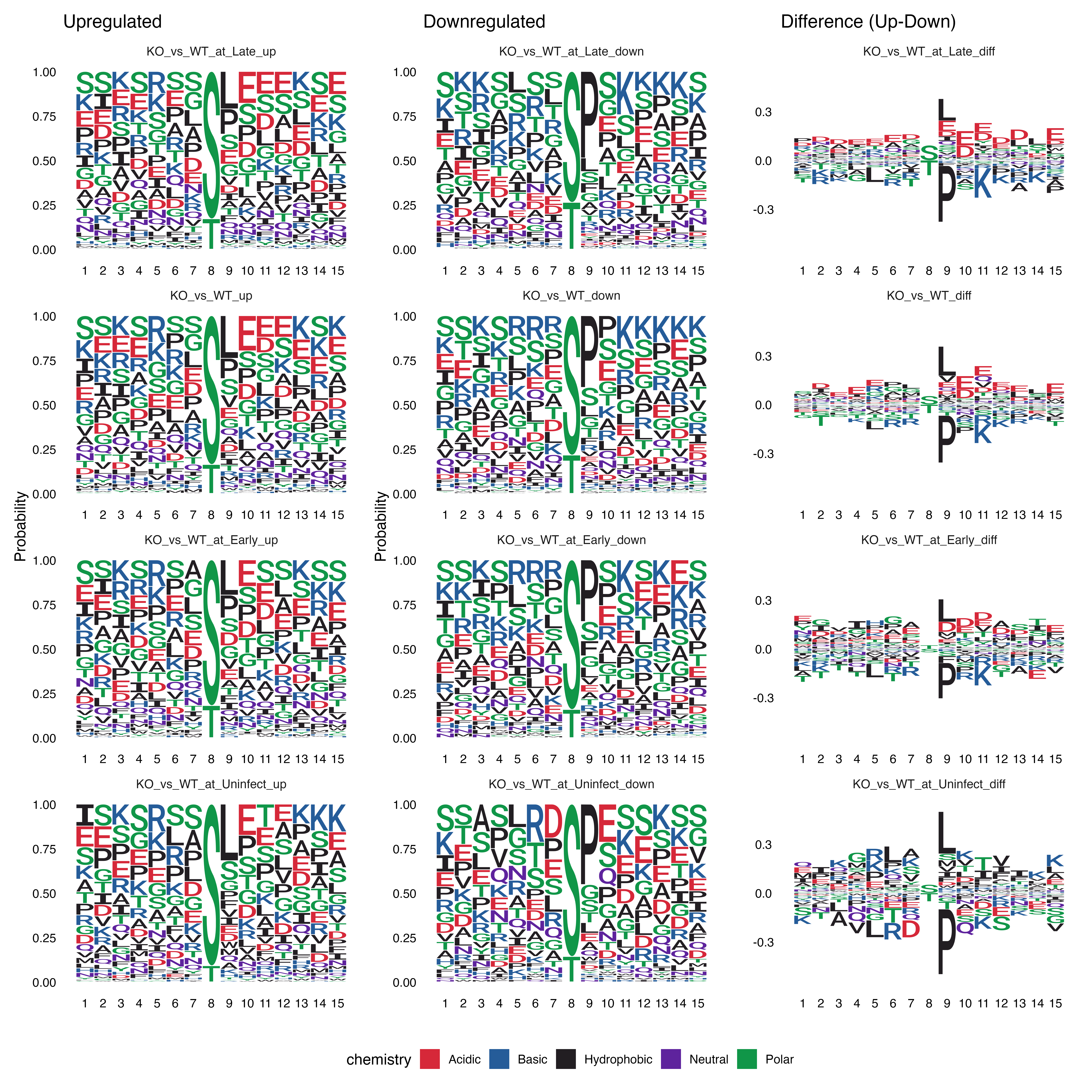
(ref:fig5seqlogoST)

Tables

Annotation table created from FragPipe outputs, with a set of columns required by prolfquapp

channel	Name	group	subject	CONTROL
KO_Early_1	KO_Early_1	NA	NA	NA
KO_Early_2	KO_Early_2	NA	NA	NA
KO_Late_1	KO_Late_1	NA	NA	NA
KO_Late_2	KO_Late_2	NA	NA	NA
KO_Uninfect_1	KO_Uninfect_1	NA	NA	NA
KO_Uninfect_2	KO_Uninfect_2	NA	NA	NA

Annotation table with explanatory variables and contrasts.

channel	Name	Group	ContrastName	Contrast
KO_Early_1	KO_Early_1	KO_Early	KO_vs_WT	( (G_KO_Uninfect + G_KO_Late + G_KO_Early)/3 - (G_WT_Uninfect + G_WT_Late + G_WT_Early)/3 )
KO_Early_2	KO_Early_2	KO_Early	KO_vs_WT_at_Uninfect	G_KO_Uninfect - G_WT_Uninfect
KO_Late_1	KO_Late_1	KO_Late	KO_vs_WT_at_Late	G_KO_Late - G_WT_Late
KO_Late_2	KO_Late_2	KO_Late	KO_vs_WT_at_Early	G_KO_Early - G_WT_Early
KO_Uninfect_1	KO_Uninfect_1	KO_Uninfect	NA	NA
KO_Uninfect_2	KO_Uninfect_2	KO_Uninfect	NA	NA

Match rates between PTM sites and proteins.

Contrast	Total Sites	Matched Sites	Match Rate
KO_vs_WT	21733	21000	96.6
KO_vs_WT_at_Early	21733	21000	96.6
KO_vs_WT_at_Late	21733	21000	96.6
KO_vs_WT_at_Uninfect	21733	21000	96.6

Consensus phosphorylation motifs of representative serine/threonine kinases. Motifs are defined relative to the phosphorylated residue (S/T at position 0). X = any residue; positions are relative to the phospho-acceptor serine/threonine (S/T).

Kinase	Consensus_motif	Positional_notes
PKA/PKG	R-R-X-S/T	Arg at -3 and -2
PKC	R-X-S/T-X-R	Arg at -3 and +2
CK2	S/T-X-X-E/D	Acidic residue at +3
MAPK	P-X-S/T-P	Pro at -2 and +1

Number of significantly regulated sites, for each contrast, amino acid residue, and up- or down-regulation.

contrast	regulation	modAA	Freq
KO_vs_WT	downregulated	S	309
KO_vs_WT_at_Early	downregulated	S	170
KO_vs_WT_at_Late	downregulated	S	221
KO_vs_WT_at_Uninfect	downregulated	S	72
KO_vs_WT	upregulated	S	499
KO_vs_WT_at_Early	upregulated	S	236
KO_vs_WT_at_Late	upregulated	S	315
KO_vs_WT_at_Uninfect	upregulated	S	140
KO_vs_WT	downregulated	T	85
KO_vs_WT_at_Early	downregulated	T	32
KO_vs_WT_at_Late	downregulated	T	79
KO_vs_WT_at_Uninfect	downregulated	T	12
KO_vs_WT	upregulated	T	97
KO_vs_WT_at_Early	upregulated	T	52
KO_vs_WT_at_Late	upregulated	T	65
KO_vs_WT_at_Uninfect	upregulated	T	14
KO_vs_WT	downregulated	Y	10
KO_vs_WT_at_Early	downregulated	Y	7
KO_vs_WT_at_Late	downregulated	Y	5
KO_vs_WT_at_Uninfect	downregulated	Y	1
KO_vs_WT	upregulated	Y	42
KO_vs_WT_at_Early	upregulated	Y	43
KO_vs_WT_at_Late	upregulated	Y	41
KO_vs_WT_at_Uninfect	upregulated	Y	1