Quality Control & Sample Size Estimation

Introduction

Workunit:
Project:
Order :

We did run your samples through the same analysis pipeline, which will be applied in the main experiment. This document summarizes the protein variability to asses the reproducibility of the biological samples and estimates the sample sizes needed for the main experiment.

Quality Control: Identifications and Quantifications

Here we summarize the number of proteins measured in the QC experiment. Depending on the type of your sample (e.g., pull-down, supernatant, whole cell lysate) we observe some dozens up to a few thousands of proteins. While the overall number of proteins can highly vary depending of the type of experiment, it is crucial that the number of proteins between your biological replicates is similar (reproducibility).

Nr of proteins detected in all samples.
NR.isotope	NR.protein_Id	NR.peptide_Id
light	163	1258

(ref:hierarchyCountsSampleBarplot) Number of quantified proteins per sample.

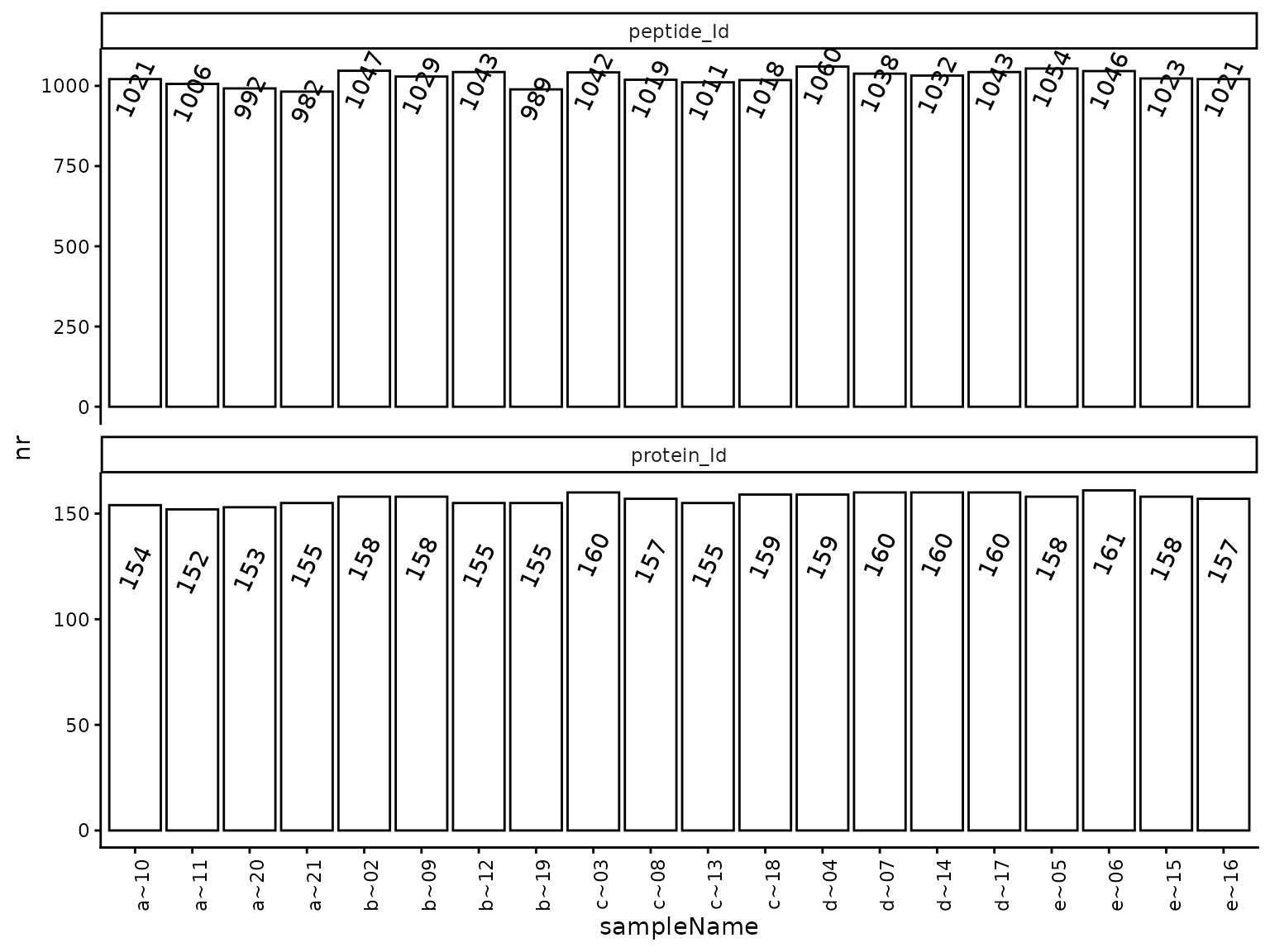
(ref:hierarchyCountsSampleBarplot)

(ref:hierarchyCountsSample) The plot shows the relationships between sets of proteins through their intersections, as well as the size of each set. The elements that are present in each intersection are shown as circles or dots in the matrix, and the size of each set is represented by the height of the corresponding row.

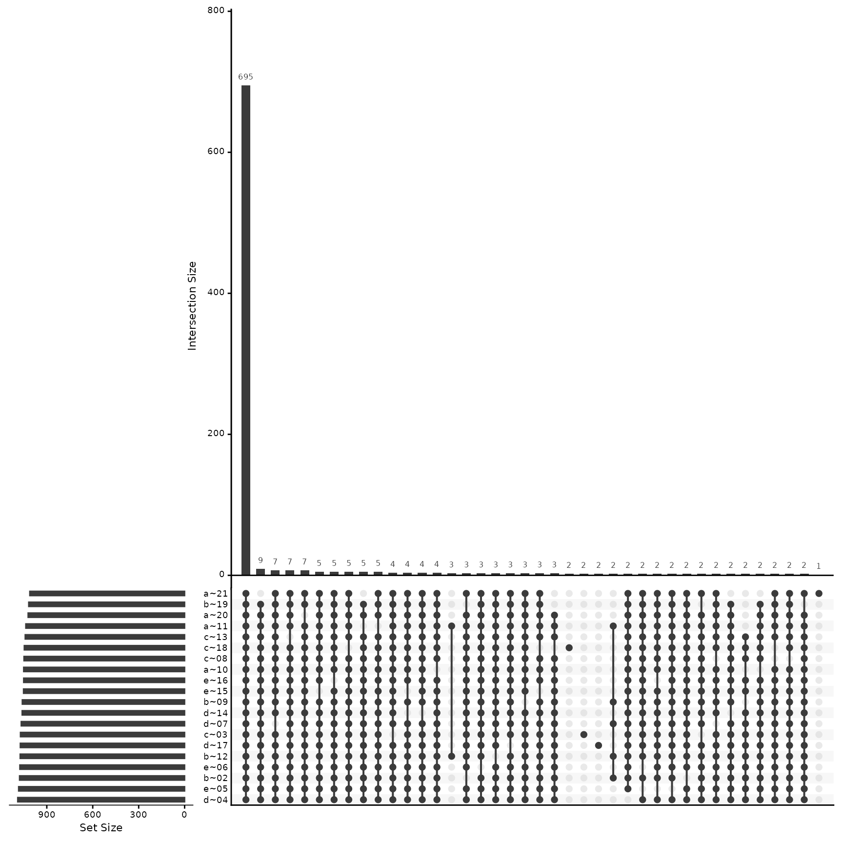
(ref:hierarchyCountsSample)

Ideally, we identify each protein in all of the samples. However, because of the limit of detection (LOD) low-intensity proteins might not be observed in all samples. Ideally, the LOD should be the only source of missingness in biological replicates. The following figures help us to verify the reproducibility of the measurement at the level of missing data.

(ref:missingFigIntensityHistorgram) Top - intensity distribution of proteins with 0, 1 etc. missing values. B - number of proteins with 0, 1, 2 etc. missing value.

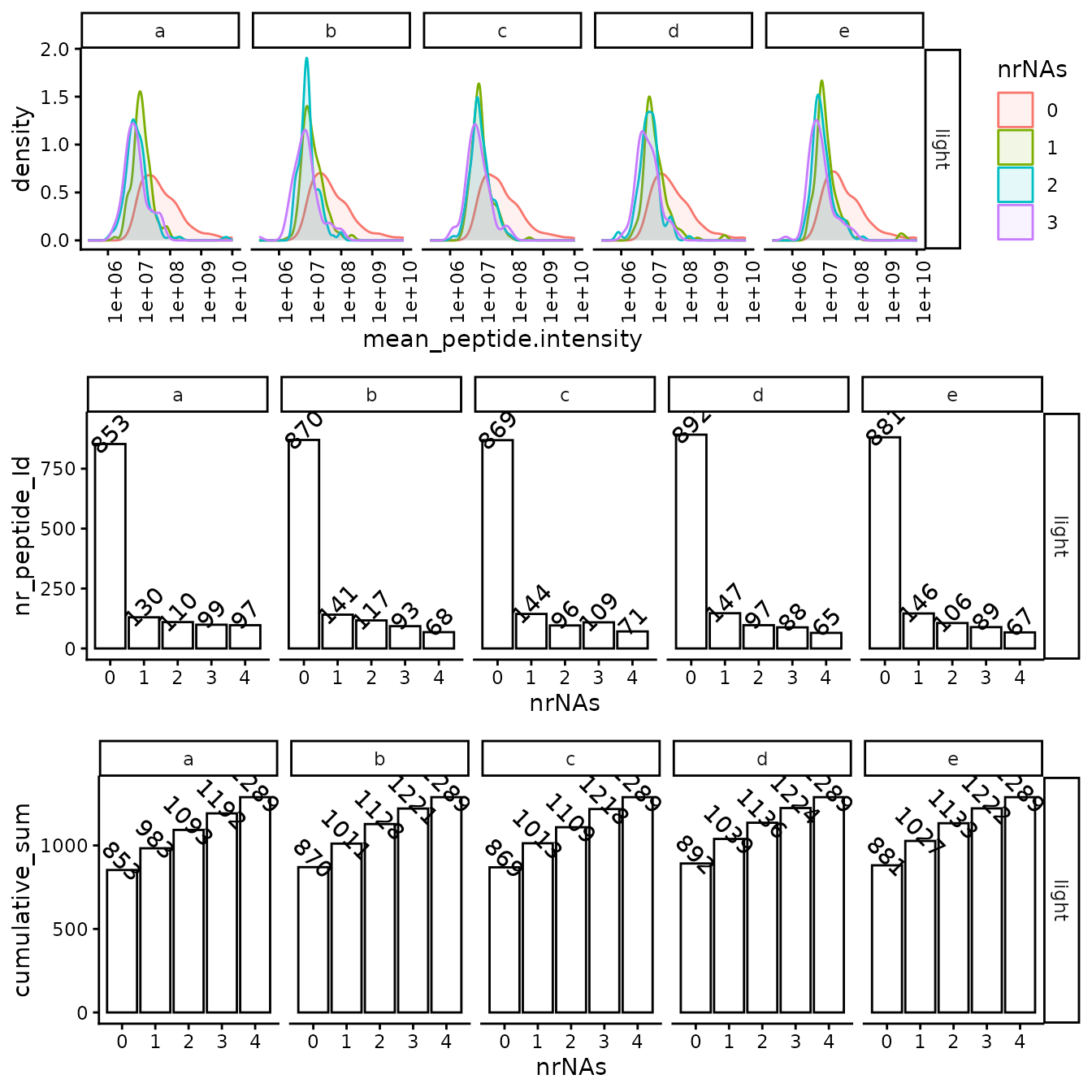
(ref:missingFigIntensityHistorgram)

(ref:missingnessHeatmap) Heatmap of missing protein quantifications clustered by sample.

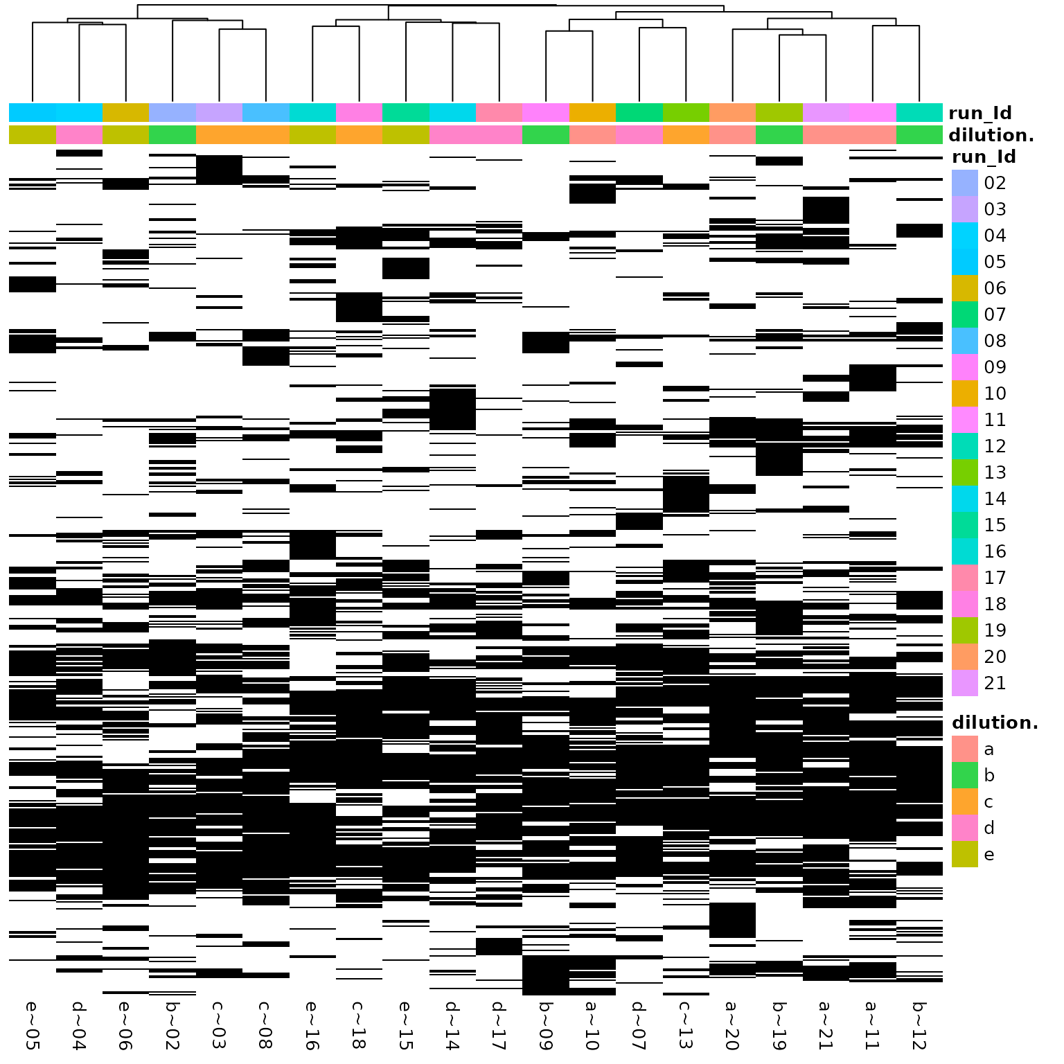
(ref:missingnessHeatmap)

Variablity of the raw intensities

Without applying any intensity scaling and data preprocessing, the protein intensities in all samples should be similar. To assess this we plotted the distribution of the protein intensities in the samples (Figure @ref(fig:plotDistributions)) as well as the distribution of the coefficient of variation CV for all proteins in the samples (Figure @ref(fig:intensityDistribution)). Table @ref(tab:printTable) summarises the CV.

(ref:plotDistributions) Density plot of protein level Coefficient of Variations (CV).

(ref:plotDistributions)

Summary of the coefficient of variation (CV) at the 50th, 60th, 70th, 80th and 90th percentile.
probs	e	a	b	c	d	All
0.5	19.84150	17.19356	18.27516	18.27122	18.34845	22.33335
0.6	22.59270	20.18408	21.12670	21.04286	21.46828	25.65000
0.7	25.93725	23.50090	24.87077	24.89460	25.27467	30.15509
0.8	32.05808	28.34406	30.73163	31.43322	31.74267	35.63108
0.9	42.68712	41.05645	40.27659	43.83096	40.84628	43.73533

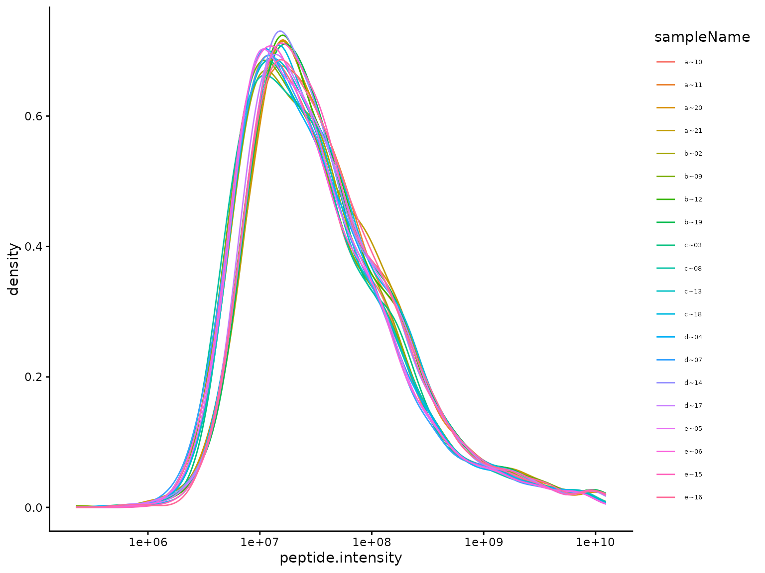
Distribution of unnormalized intensities.

Variability of transformed intensities

We applied the vsn::justvsn normalization to the data, which should remove systematic differences among the samples and reduce the variance within the groups (Figure @ref(fig:plotTransformedIntensityDistributions)). Because of this transformation, we can’t report $CV's$ anymore but report standard deviations ( $sd$ ). Figure @ref(fig:sdviolinplots) shows the distribution of the protein standard deviations while Figure @ref(fig:sdecdf) shows the empirical cumulative distribution function ( $ecdf$ ). Table @ref(tab:printSDTable) summarises the $sd$ . The heatmap in Figure @ref(fig:correlationHeat) shows the correlation among the QC samples.

(ref:plotTransformedIntensityDistributions) protein intensity distribution after transformation.

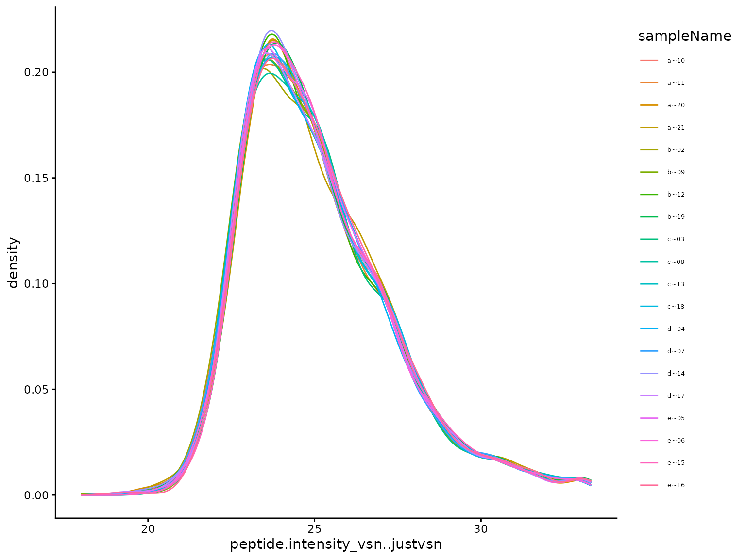
(ref:plotTransformedIntensityDistributions)

(ref:correlationHeat) Heatmap of protein intensity correlation between samples.

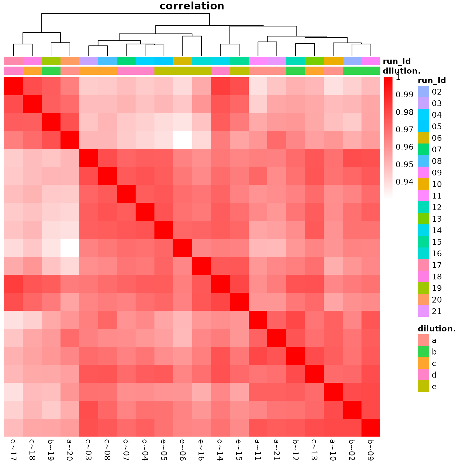
(ref:correlationHeat)

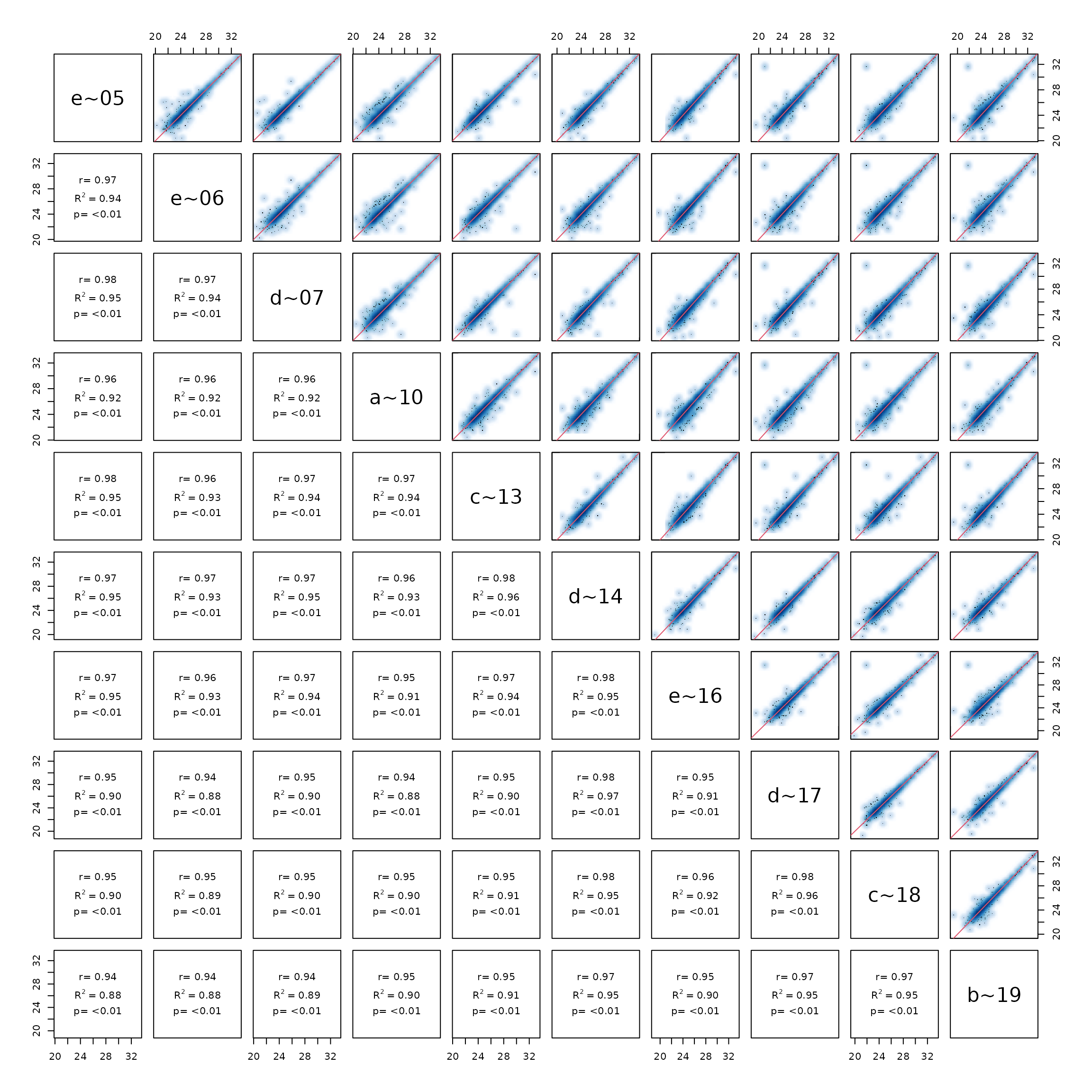
Pairsplot - scatterplot of samples.

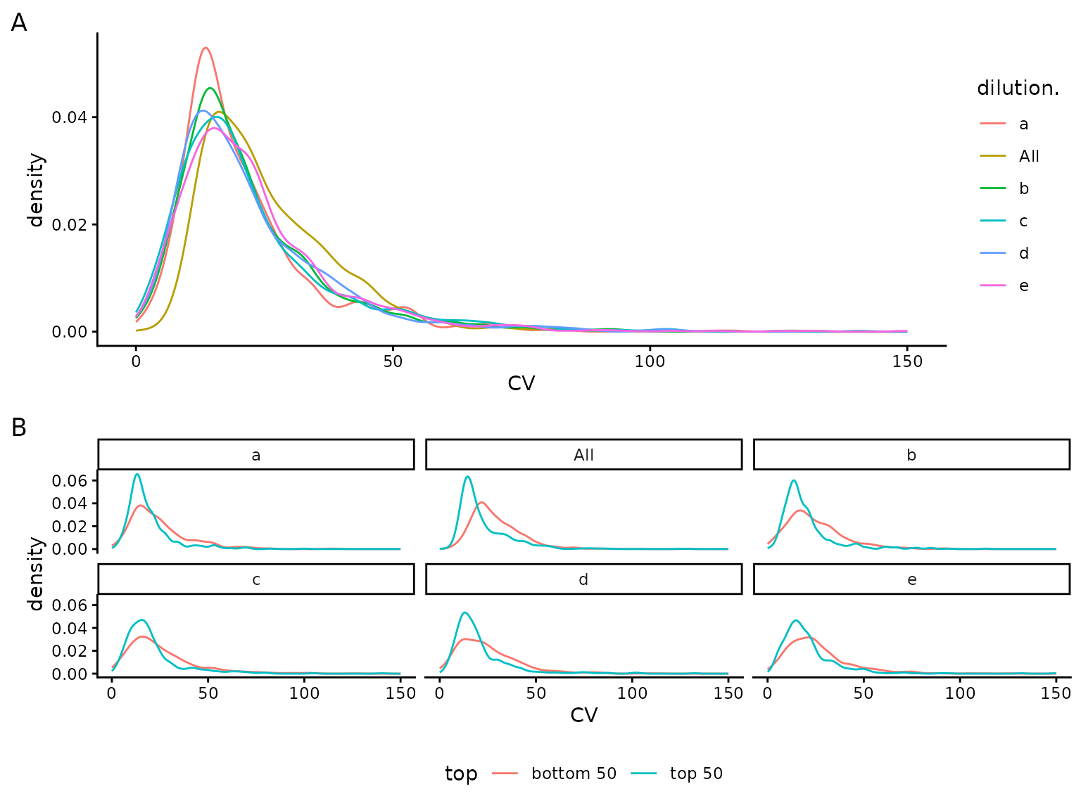
## NULL

(ref:sdviolinplots) Visualization of protein standard deviations. A) all. B) - for low (bottom 50) and high intensity (top 50).

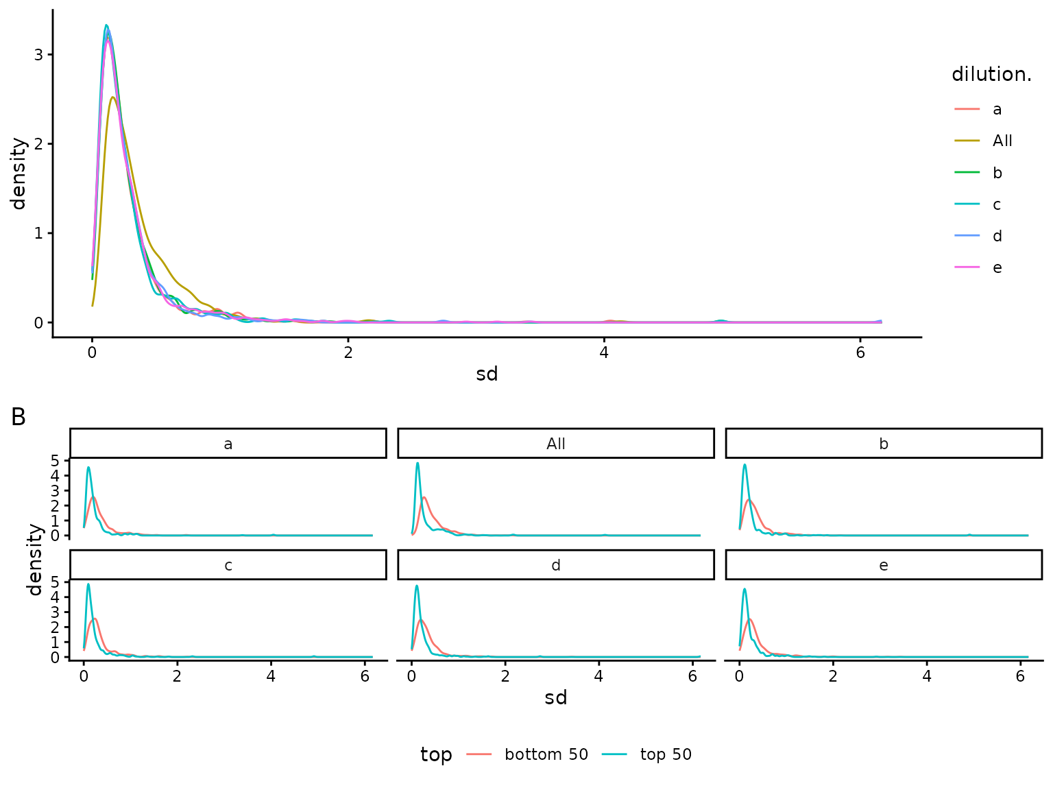
(ref:sdviolinplots)

(ref:sdecdf) Visualization of protein standard deviations as empirical cumulative distribution function. A) all. B) - for low (bottom 50) and high intensity (top 50).

## NULL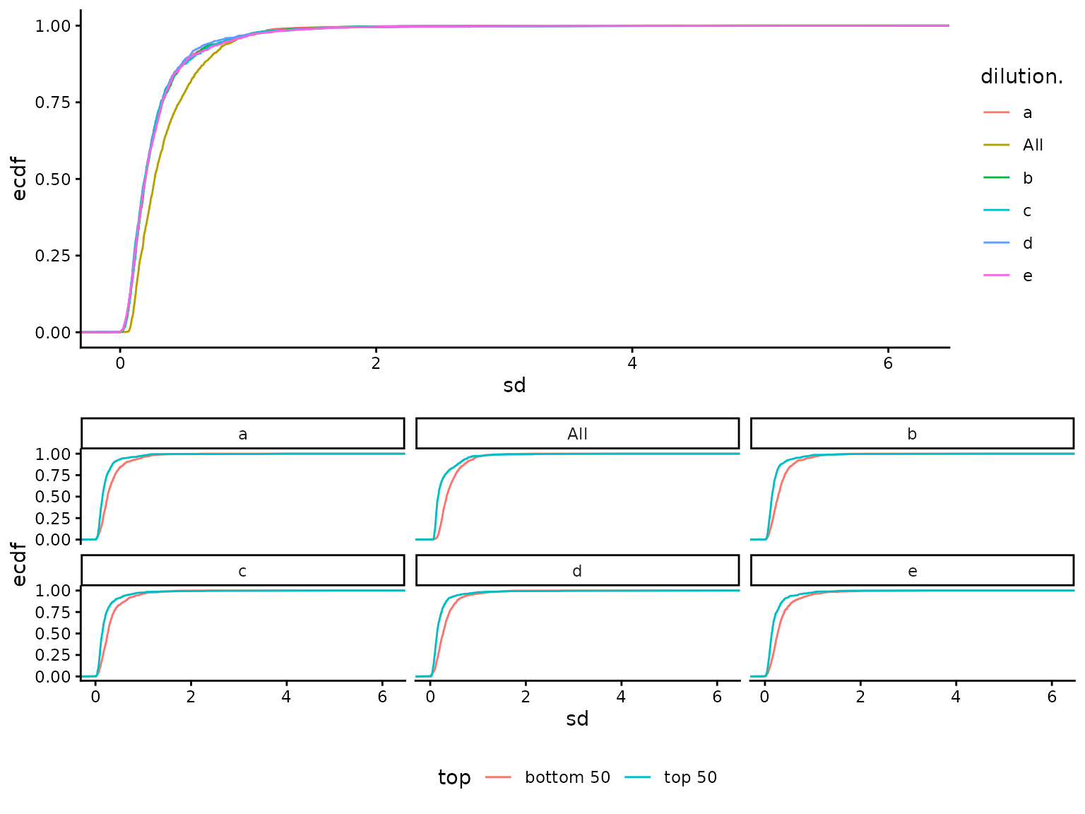

(ref:sdecdf)

Summary of the distribution of standard deviations at the 50th, 60th, 70th, 80th and 90th percentile.
probs	e	a	b	c	d	All
0.5	0.1970862	0.1946647	0.1944917	0.1910686	0.1980979	0.2702206
0.6	0.2421660	0.2369077	0.2377510	0.2362158	0.2395528	0.3311495
0.7	0.3013293	0.2932444	0.2978505	0.2849253	0.2955599	0.4071946
0.8	0.3795823	0.3715429	0.3863823	0.3637895	0.3720552	0.5257856
0.9	0.5626683	0.5540956	0.5632134	0.5814590	0.5437999	0.7131470

(ref:overviewHeat) Sample and protein Heatmap.

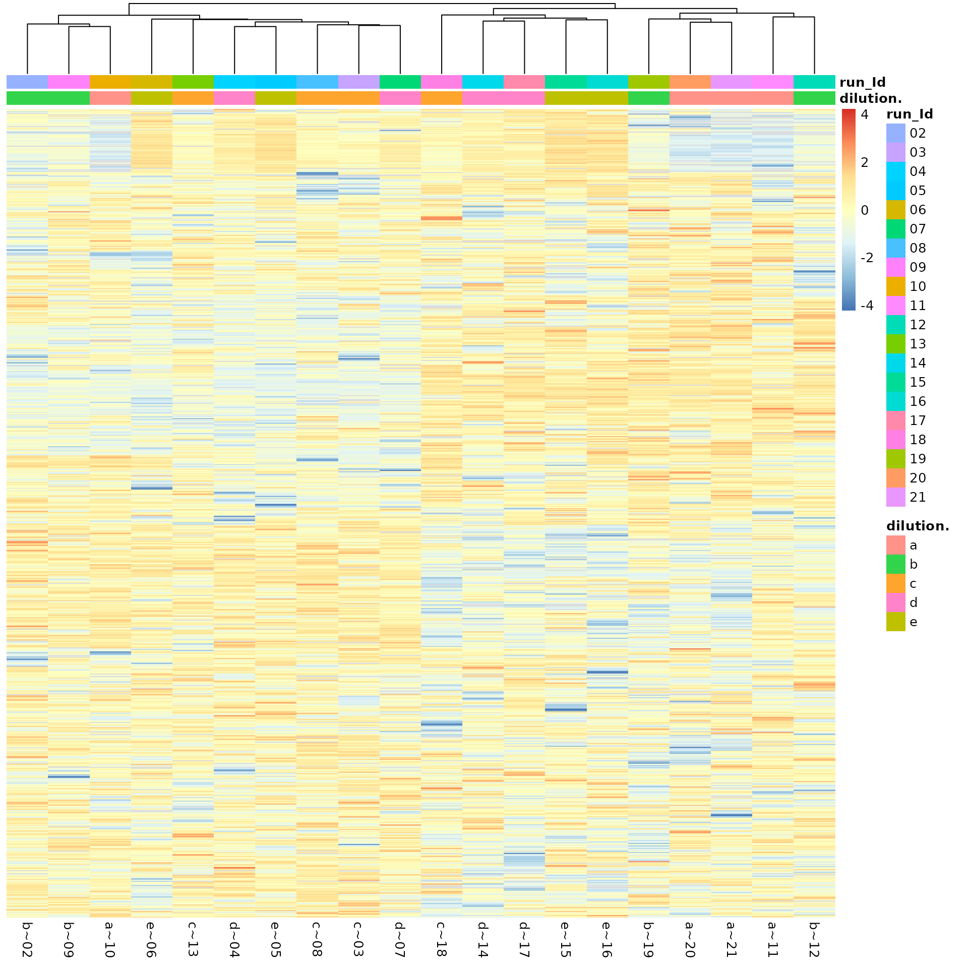
(ref:overviewHeat)

Sample Size Calculation

In the previous section, we estimated the protein variance using the QC samples. Figure @ref(fig:sdviolinplots) shows the distribution of the standard deviations. We are using this information, as well as some typical values for the size and the power of the test to estimate the required sample sizes for your main experiment.

An important factor in estimating the sample sizes is the smallest effect size (difference) you are interested in detecting between two conditions, e.g. a reference and a treatment. Smaller biologically significant effect sizes require more samples to obtain a statistically significant result. Typical $log_2$ fold change thresholds are $0.59, 1, 2$ which correspond to a fold change of $1.5, 2, 4$ .

Table @ref(tab:sampleSize) and Figure @ref(fig:figSampleSize) summarizes how many samples are needed to detect a fold change of $0.5, 1, 2$ at a confidence level of $95\%$ and power of $80\%$ , for $50, 60, 70, 80$ and $90\%$ percent of the measured proteins.

(ref:figSampleSize) Graphical representation of the sample size needed to detect a log fold change greater than delta with a significance level of $0.05$ and power 0.8 when using a t-test to compare means, in $X\%$ of proteins (x - axis).

(ref:figSampleSize)

Sample size needed to detect a difference log fold change greater than delta with a significance level of 0.05 and power 0.8 when using a t-test to compare means.
probs	sdtrimmed	dilution.	delta = 0.59	delta = 1	delta = 2
0.50	0.1970862	e	4	3	2
0.75	0.3302951	e	7	4	2
0.50	0.1946647	a	4	3	2
0.75	0.3276262	a	6	4	2
0.50	0.1944917	b	4	3	2
0.75	0.3327904	b	7	4	2
0.50	0.1910686	c	3	3	2
0.75	0.3177703	c	6	3	2
0.50	0.1980979	d	4	3	2
0.75	0.3266973	d	6	4	2
0.50	0.2702206	All	5	3	2
0.75	0.4619799	All	11	5	3

The power of a test is $1-\beta$ , where $\beta$ is the probability of a Type 2 error (failing to reject the null hypothesis when the alternative hypothesis is true). In other words, if you have a $20\%$ chance of failing to detect a real difference, then the power of your test is $80\%$ .

The confidence level is equal to $1 - \alpha$ , where $\alpha$ is the probability of making a Type 1 Error. That is, alpha represents the chance of a falsely rejecting $H_0$ and picking up a false-positive effect. Alpha is usually set at $5\%$ significance level, for a $95\%$ confidence level.

Fold change: Suppose you are comparing a treatment group to a placebo group, and you will be measuring some continuous response variable which, you hypothesize, will be affected by the treatment. We can consider the mean response in the treatment group, $\mu_1$ , and the mean response in the placebo group, $\mu_2$ . We can then define $\Delta = \mu_1 - \mu_2$ as the mean difference. The smaller the difference you want to detect, the larger the required sample size.

Appendix

Mapping of raw file names to sample names used throughout this report.
raw.file	sampleName	dilution.	run_Id
b03_10_150304_human_ecoli_a_3ul_3um_column_95_hcd_ot_2hrs_30b_9b	a~10	a	10
b03_11_150304_human_ecoli_a_3ul_3um_column_95_hcd_ot_2hrs_30b_9b	a~11	a	11
b03_20_150304_human_ecoli_a_3ul_3um_column_95_hcd_ot_2hrs_30b_9b	a~20	a	20
b03_21_150304_human_ecoli_a_3ul_3um_column_95_hcd_ot_2hrs_30b_9b	a~21	a	21
b03_02_150304_human_ecoli_b_3ul_3um_column_95_hcd_ot_2hrs_30b_9b	b~02	b	02
b03_09_150304_human_ecoli_b_3ul_3um_column_95_hcd_ot_2hrs_30b_9b	b~09	b	09
b03_12_150304_human_ecoli_b_3ul_3um_column_95_hcd_ot_2hrs_30b_9b	b~12	b	12
b03_19_150304_human_ecoli_b_3ul_3um_column_95_hcd_ot_2hrs_30b_9b	b~19	b	19
b03_03_150304_human_ecoli_c_3ul_3um_column_95_hcd_ot_2hrs_30b_9b	c~03	c	03
b03_08_150304_human_ecoli_c_3ul_3um_column_95_hcd_ot_2hrs_30b_9b	c~08	c	08
b03_13_150304_human_ecoli_c_3ul_3um_column_95_hcd_ot_2hrs_30b_9b	c~13	c	13
b03_18_150304_human_ecoli_c_3ul_3um_column_95_hcd_ot_2hrs_30b_9b	c~18	c	18
b03_04_150304_human_ecoli_d_3ul_3um_column_95_hcd_ot_2hrs_30b_9b	d~04	d	04
b03_07_150304_human_ecoli_d_3ul_3um_column_95_hcd_ot_2hrs_30b_9b	d~07	d	07
b03_14_150304_human_ecoli_d_3ul_3um_column_95_hcd_ot_2hrs_30b_9b	d~14	d	14
b03_17_150304_human_ecoli_d_3ul_3um_column_95_hcd_ot_2hrs_30b_9b	d~17	d	17
b03_05_150304_human_ecoli_e_3ul_3um_column_95_hcd_ot_2hrs_30b_9b	e~05	e	05
b03_06_150304_human_ecoli_e_3ul_3um_column_95_hcd_ot_2hrs_30b_9b	e~06	e	06
b03_15_150304_human_ecoli_e_3ul_3um_column_95_hcd_ot_2hrs_30b_9b	e~15	e	15
b03_16_150304_human_ecoli_e_3ul_3um_column_95_hcd_ot_2hrs_30b_9b	e~16	e	16

Number of quantified proteins per sample.
isotope	sampleName	protein_Id	peptide_Id
light	a~10	154	1021
light	a~11	152	1006
light	a~20	153	992
light	a~21	155	982
light	b~02	158	1047
light	b~09	158	1029
light	b~12	155	1043
light	b~19	155	989
light	c~03	160	1042
light	c~08	157	1019
light	c~13	155	1011
light	c~18	159	1018
light	d~04	159	1060
light	d~07	160	1038
light	d~14	160	1032
light	d~17	160	1043
light	e~05	158	1054
light	e~06	161	1046
light	e~15	158	1023
light	e~16	157	1021