Pipeline Demo: Fit → Write → Score → Aggregate

This vignette demonstrates the pipeline architecture for benchmarking. Instead of fitting models and benchmarking in one monolithic script, the workflow is split into three decoupled steps:

Fit — fit models and compute contrasts, write standardized output files
Score — load contrast result files, create Benchmark objects, compute metrics
Aggregate — collect benchmark summaries across methods for comparison

Each fitting step produces a directory with contrasts.tsv + metadata.yaml. This enables a future Snakemake pipeline: for each dataset × method → fit → score → aggregate.

conflicted::conflict_prefer("filter", "dplyr")

Shared Data Preparation

This section is identical to BenchmarkingIonstarData.Rmd — load and normalize the IonStar dataset, aggregate peptides to proteins via median polish.

datadir <- file.path(find.package("prolfquadata"), "quantdata")
inputMQfile <- file.path(datadir, "MAXQuant_IonStar2018_PXD003881.zip")
inputAnnotation <- file.path(datadir, "annotation_Ionstar2018_PXD003881.xlsx")

mqdata <- list()
mqdata$data <- prolfquapp::tidyMQ_Peptides(inputMQfile)
mqdata$config <- prolfqua::create_config_MQ_peptide()

annotation <- readxl::read_xlsx(inputAnnotation)
res <- dplyr::inner_join(mqdata$data, annotation, by = "raw.file")

mqdata$config$table$factors[["dilution."]] <- "sample"
mqdata$config$table$factors[["run_Id"]] <- "run_ID"
mqdata$config$table$factorDepth <- 1
mqdata$data <- prolfqua::setup_analysis(res, mqdata$config)

lfqdata <- prolfqua::LFQData$new(mqdata$data, mqdata$config)
lfqdata$data <- lfqdata$data |> dplyr::filter(!grepl("^REV__|^CON__", protein_Id))
lfqdata$filter_proteins_by_peptide_count()
lfqdata$remove_small_intensities()

# Normalize using HUMAN subset
tr <- lfqdata$get_Transformer()
subset_h <- lfqdata$get_copy()
subset_h$data <- subset_h$data |> dplyr::filter(grepl("HUMAN", protein_Id))
subset_h <- subset_h$get_Transformer()$log2()$lfq
lfqdataNormalized <- tr$log2()$robscale_subset(lfqsubset = subset_h, preserveMean = FALSE)$lfq

# Median polish aggregation
lfqAggMedpol <- lfqdataNormalized$get_Aggregator()
lfqAggMedpol$medpolish()
protLFQ <- lfqAggMedpol$lfq_agg

relevantContrasts <- c(
  "dilution_(9/7.5)_1.2"    = "dilution.e - dilution.d",
  "dilution_(7.5/6)_1.25"   = "dilution.d - dilution.c",
  "dilution_(6/4.5)_1.3(3)" = "dilution.c - dilution.b",
  "dilution_(4.5/3)_1.5"    = "dilution.b - dilution.a"
)

output_base <- tempfile("benchmark_pipeline_")
dir.create(output_base)
message("Pipeline output directory: ", output_base)

Step 1: Fit & Write

Each method fits models, computes contrasts, and writes the results using write_contrast_results(). This produces a contrasts.tsv + metadata.yaml per method.

Method: Linear model (lm)

lmmodel <- paste0(protLFQ$config$table$get_response(), " ~ dilution.")
modelFunction <- prolfqua::strategy_lm(lmmodel, model_name = "Model")
modLinearProt <- prolfqua::build_model(protLFQ$data, modelFunction)

contrProt <- prolfqua::Contrasts$new(modLinearProt, relevantContrasts)
contrast_data_lm <- contrProt$get_contrasts()

write_contrast_results(
  data = contrast_data_lm,
  path = file.path(output_base, "ionstar_lm"),
  metadata = list(
    dataset = "ionstar_maxquant",
    method = "prolfqua_lm",
    method_description = "Linear model on median-polished proteins",
    input_file = "MAXQuant_IonStar2018_PXD003881.zip/peptides.txt",
    aggregation = "median_polish",
    normalization = "robscale",
    software_version = paste0("prolfqua ", packageVersion("prolfqua")),
    date = as.character(Sys.Date()),
    contrasts = names(relevantContrasts),
    ground_truth = list(
      id_column = "protein_id",
      positive = list(label = "ECOLI", pattern = "ECOLI"),
      negative = list(label = "HUMAN", pattern = "HUMAN")
    )
  )
)

Method: Moderated linear model (lm + moderation)

contrProtModerated <- prolfqua::ContrastsModerated$new(contrProt)
contrast_data_lm_mod <- contrProtModerated$get_contrasts()

write_contrast_results(
  data = contrast_data_lm_mod,
  path = file.path(output_base, "ionstar_lm_mod"),
  metadata = list(
    dataset = "ionstar_maxquant",
    method = "prolfqua_lm_mod",
    method_description = "Linear model with variance moderation on median-polished proteins",
    input_file = "MAXQuant_IonStar2018_PXD003881.zip/peptides.txt",
    aggregation = "median_polish",
    normalization = "robscale",
    software_version = paste0("prolfqua ", packageVersion("prolfqua")),
    date = as.character(Sys.Date()),
    contrasts = names(relevantContrasts),
    ground_truth = list(
      id_column = "protein_id",
      positive = list(label = "ECOLI", pattern = "ECOLI"),
      negative = list(label = "HUMAN", pattern = "HUMAN")
    )
  )
)

Method: Imputation (missing value model)

contrImp <- prolfqua::ContrastsMissing$new(protLFQ, relevantContrasts)
contrast_data_imp <- contrImp$get_contrasts()

write_contrast_results(
  data = contrast_data_imp,
  path = file.path(output_base, "ionstar_missing"),
  metadata = list(
    dataset = "ionstar_maxquant",
    method = "prolfqua_missing",
    method_description = "Median polish and missingness modelling",
    input_file = "MAXQuant_IonStar2018_PXD003881.zip/peptides.txt",
    aggregation = "median_polish",
    normalization = "robscale",
    software_version = paste0("prolfqua ", packageVersion("prolfqua")),
    date = as.character(Sys.Date()),
    contrasts = names(relevantContrasts),
    ground_truth = list(
      id_column = "protein_id",
      positive = list(label = "ECOLI", pattern = "ECOLI"),
      negative = list(label = "HUMAN", pattern = "HUMAN")
    )
  )
)

Method: Merged (lm + imputation, moderated)

all_merged <- prolfqua::merge_contrasts_results(prefer = contrProt, add = contrImp)
merged_mod <- prolfqua::ContrastsModerated$new(all_merged$merged)
contrast_data_merged <- merged_mod$get_contrasts()

write_contrast_results(
  data = contrast_data_merged,
  path = file.path(output_base, "ionstar_merged"),
  metadata = list(
    dataset = "ionstar_maxquant",
    method = "prolfqua_merged",
    method_description = "Merge of lm moderated and imputed contrasts",
    input_file = "MAXQuant_IonStar2018_PXD003881.zip/peptides.txt",
    aggregation = "median_polish",
    normalization = "robscale",
    software_version = paste0("prolfqua ", packageVersion("prolfqua")),
    date = as.character(Sys.Date()),
    contrasts = names(relevantContrasts),
    ground_truth = list(
      id_column = "protein_id",
      positive = list(label = "ECOLI", pattern = "ECOLI"),
      negative = list(label = "HUMAN", pattern = "HUMAN")
    )
  )
)

Inspect output files

list.files(output_base, recursive = TRUE)

## [1] "ionstar_lm_mod/contrasts.tsv"  "ionstar_lm_mod/metadata.yaml" 
## [3] "ionstar_lm/contrasts.tsv"      "ionstar_lm/metadata.yaml"     
## [5] "ionstar_merged/contrasts.tsv"  "ionstar_merged/metadata.yaml" 
## [7] "ionstar_missing/contrasts.tsv" "ionstar_missing/metadata.yaml"

lm_data <- utils::read.delim(
  file.path(output_base, "ionstar_lm", "contrasts.tsv"),
  nrows = 5
)
knitr::kable(lm_data, caption = "First 5 rows of ionstar_lm/contrasts.tsv")

First 5 rows of ionstar_lm/contrasts.tsv
modelName	protein_id	contrast	sigma	df	log_fc	p_value_adjusted	std.error	t_statistic	p_value	conf.low	conf.high	avgAbd
WaldTest	sp\|A0AVT1\|UBA6_HUMAN	dilution_(9/7.5)_1.2	0.1350528	15	-0.0525662	0.9440215	0.0954967	-0.5504504	0.5901146	-0.2561127	0.1509803	-1.3494300
WaldTest	sp\|A0AVT1\|UBA6_HUMAN	dilution_(7.5/6)_1.25	0.1350528	15	-0.0902570	0.8752505	0.0954967	-0.9451316	0.3595683	-0.2938035	0.1132895	-1.2780184
WaldTest	sp\|A0AVT1\|UBA6_HUMAN	dilution_(6/4.5)_1.3(3)	0.1350528	15	-0.0494793	0.9647062	0.0954967	-0.5181250	0.6119287	-0.2530257	0.1540672	-1.2081503
WaldTest	sp\|A0AVT1\|UBA6_HUMAN	dilution_(4.5/3)_1.5	0.1350528	15	0.0837284	0.8888834	0.0954967	0.8767667	0.3944387	-0.1198181	0.2872748	-1.2252748
WaldTest	sp\|A0FGR8\|ESYT2_HUMAN	dilution_(9/7.5)_1.2	0.0854070	15	-0.0533352	0.8725464	0.0603918	-0.8831531	0.3910883	-0.1820574	0.0753869	-0.3097215

cat(readLines(file.path(output_base, "ionstar_lm", "metadata.yaml")), sep = "\n")

## dataset: ionstar_maxquant
## method: prolfqua_lm
## method_description: Linear model on median-polished proteins
## input_file: MAXQuant_IonStar2018_PXD003881.zip/peptides.txt
## aggregation: median_polish
## normalization: robscale
## software_version: prolfqua 1.5.0
## date: '2026-03-19'
## contrasts:
## - dilution_(9/7.5)_1.2
## - dilution_(7.5/6)_1.25
## - dilution_(6/4.5)_1.3(3)
## - dilution_(4.5/3)_1.5
## ground_truth:
##   id_column: protein_id
##   positive:
##     label: ECOLI
##     pattern: ECOLI
##   negative:
##     label: HUMAN
##     pattern: HUMAN

Step 2: Score

Load each contrast result directory with benchmark_from_file() and compute benchmark metrics. No knowledge of the fitting step is needed — the ground truth specification comes from metadata.yaml.

method_dirs <- list.dirs(output_base, recursive = FALSE)
names(method_dirs) <- basename(method_dirs)

benchmarks <- lapply(method_dirs, benchmark_from_file)

benchmarks$ionstar_lm$plot_ROC(xlim = 0.15)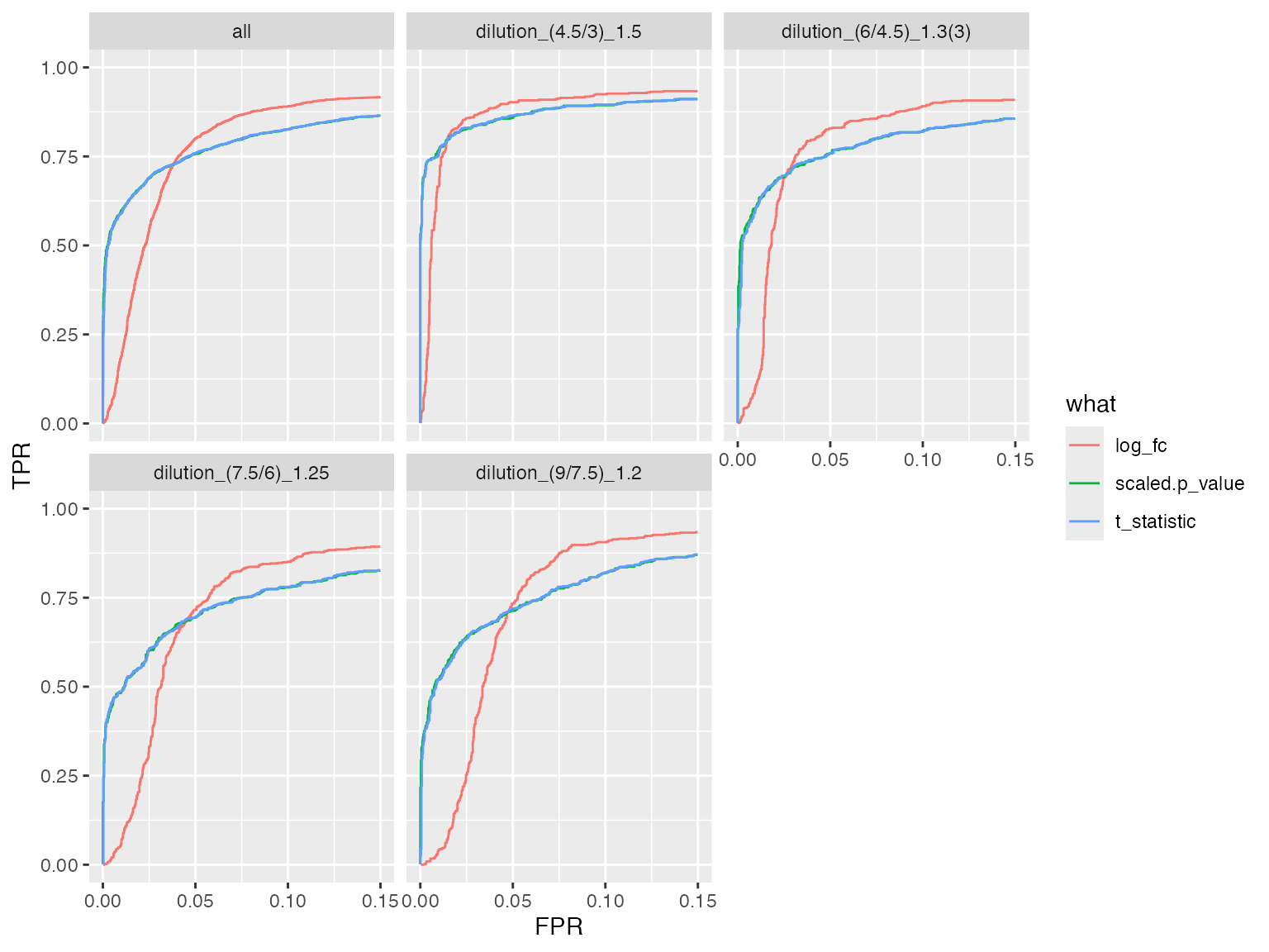

benchmarks$ionstar_lm_mod$plot_precision_recall()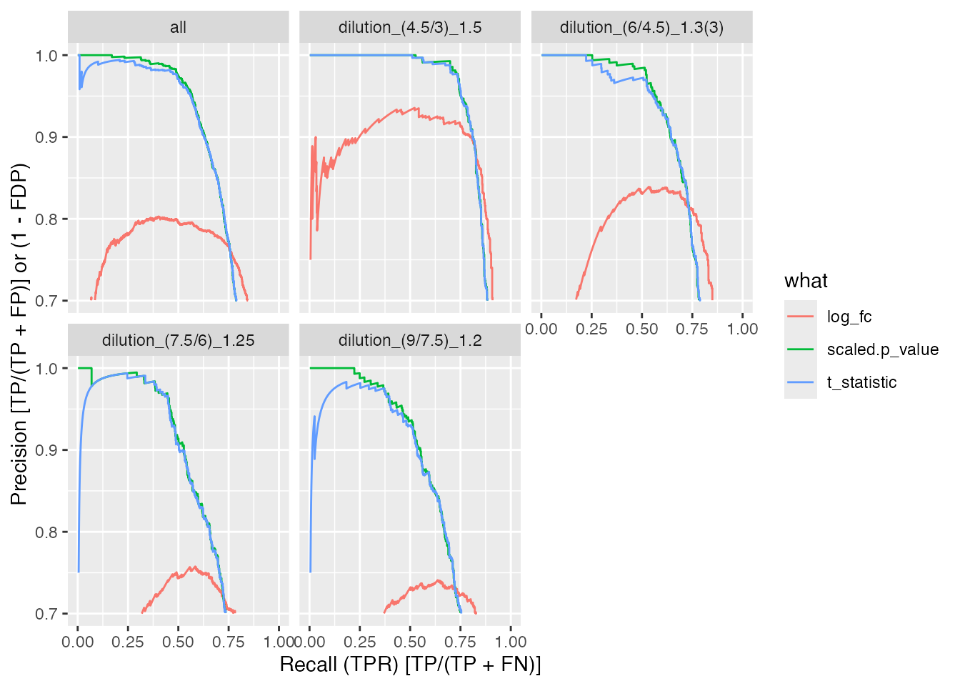

benchmarks$ionstar_merged$plot_FDRvsFDP()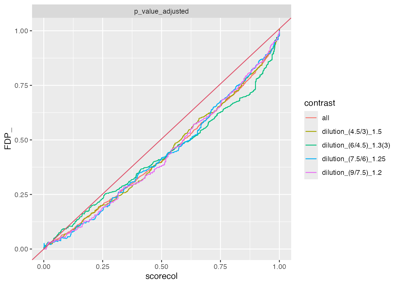

Step 3: Aggregate & Compare

Use to_summary_table() to extract metrics from each Benchmark, then combine with collect_benchmark_results() for cross-method comparison.

summary_files <- character()
for (method_name in names(benchmarks)) {
  bench <- benchmarks[[method_name]]
  bench$complete(FALSE)
  summary <- bench$to_summary_table(dataset = "ionstar_maxquant")

  outfile <- file.path(output_base, method_name, "benchmark_results.tsv")
  write_benchmark_results(summary, outfile)
  summary_files <- c(summary_files, outfile)
}

combined <- collect_benchmark_results(summary_files)
knitr::kable(
  combined |> dplyr::filter(contrast == "all"),
  caption = "Benchmark summary across methods (all contrasts pooled)",
  digits = 2
)

Benchmark summary across methods (all contrasts pooled)
model_name	model_description	dataset	contrast	score	AUC	pAUC_10	pAUC_20	AP	pAP_50	pAP_80	n_TP	n_TN	n_total	n_missing_contrasts
prolfqua_lm	Linear model on median-polished proteins	ionstar_maxquant	all	log_fc	92.74	66.98	79.21	71.37	75.69	76.58	2484	13981	16465	123
prolfqua_lm	Linear model on median-polished proteins	ionstar_maxquant	all	scaled.p_value	93.07	72.92	79.58	83.47	99.39	94.05	2484	13955	16439	123
prolfqua_lm	Linear model on median-polished proteins	ionstar_maxquant	all	t_statistic	93.06	72.78	79.54	83.12	98.72	93.60	2484	13955	16439	123
prolfqua_lm_mod	Linear model with variance moderation on median-polished proteins	ionstar_maxquant	all	log_fc	92.74	66.98	79.21	71.37	75.69	76.58	2484	13981	16465	123
prolfqua_lm_mod	Linear model with variance moderation on median-polished proteins	ionstar_maxquant	all	scaled.p_value	93.28	74.25	80.67	84.25	99.33	94.68	2484	13955	16439	123
prolfqua_lm_mod	Linear model with variance moderation on median-polished proteins	ionstar_maxquant	all	t_statistic	93.26	74.09	80.61	83.80	98.48	94.10	2484	13955	16439	123
prolfqua_merged	Merge of lm moderated and imputed contrasts	ionstar_maxquant	all	log_fc	91.98	65.68	77.62	70.86	76.50	76.99	2564	14148	16712	0
prolfqua_merged	Merge of lm moderated and imputed contrasts	ionstar_maxquant	all	scaled.p_value	92.40	72.27	78.66	82.79	99.17	93.81	2564	14148	16712	0
prolfqua_merged	Merge of lm moderated and imputed contrasts	ionstar_maxquant	all	t_statistic	92.37	72.02	78.55	82.08	97.89	92.91	2564	14148	16712	0
prolfqua_missing	Median polish and missingness modelling	ionstar_maxquant	all	log_fc	92.12	67.69	78.46	73.44	80.78	80.30	2564	14148	16712	0
prolfqua_missing	Median polish and missingness modelling	ionstar_maxquant	all	scaled.p_value	91.94	69.98	76.79	81.30	98.96	92.45	2564	14148	16712	0
prolfqua_missing	Median polish and missingness modelling	ionstar_maxquant	all	t_statistic	91.92	69.73	76.74	80.51	97.41	91.43	2564	14148	16712	0

combined_all <- combined |> dplyr::filter(contrast == "all")
long <- tidyr::pivot_longer(
  combined_all,
  cols = c("AUC", "pAUC_10", "pAUC_20", "AP", "pAP_50", "pAP_80"),
  names_to = "metric",
  values_to = "value"
)
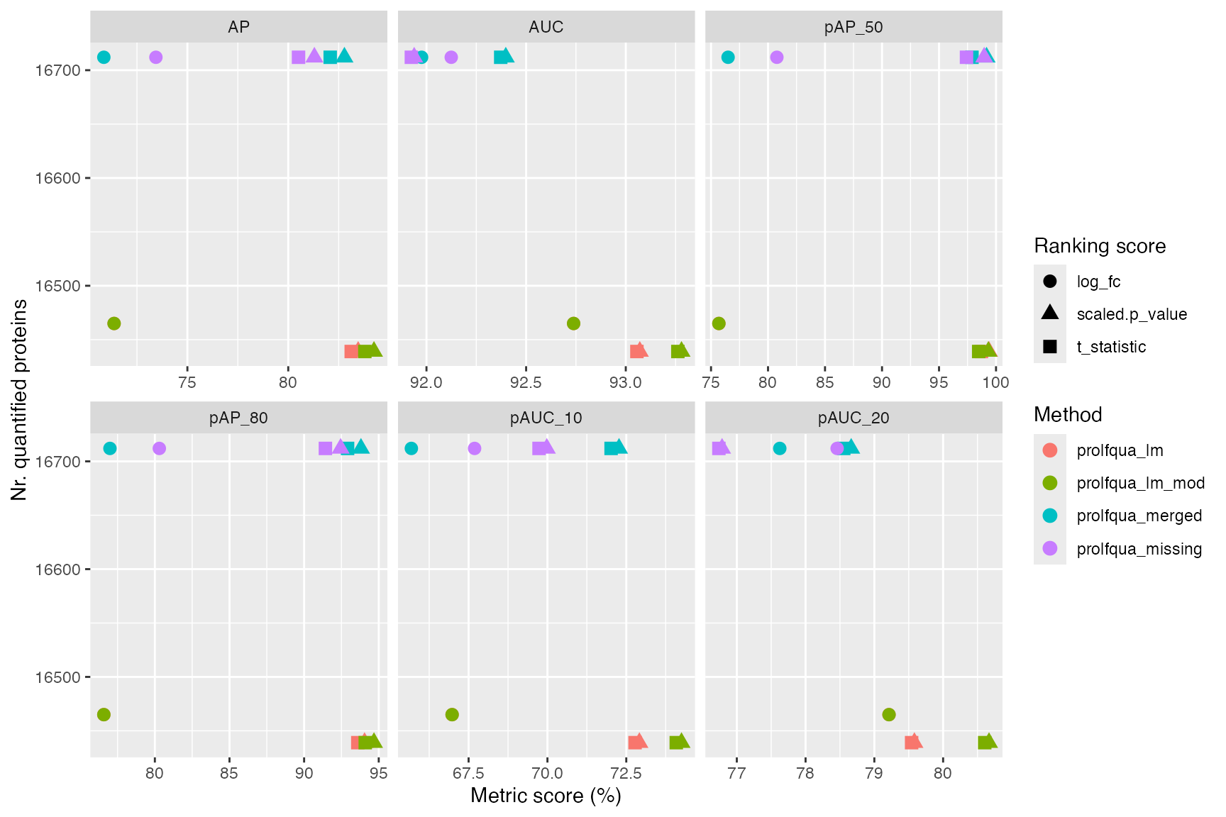
ggplot2::ggplot(
  long,
  ggplot2::aes(x = value, y = n_total, color = model_name, shape = score)
) +
  ggplot2::geom_point(size = 3) +
  ggplot2::facet_wrap(~metric, scales = "free_x") +
  ggplot2::labs(
    x = "Metric score (%)", y = "Nr. quantified proteins",
    color = "Method", shape = "Ranking score"
  )

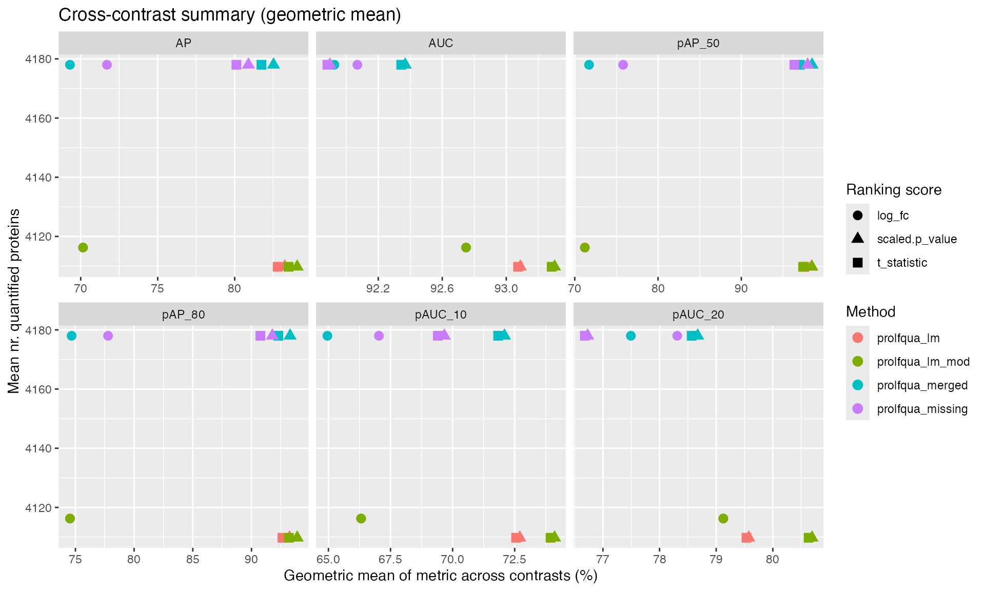
# Geometric mean across contrasts — complements the pooled "all" row above
summary_list <- lapply(benchmarks, function(b) {
  b$complete(FALSE)
  b$summary_metrics()
})
combined_summary <- dplyr::bind_rows(summary_list)

long_summary <- tidyr::pivot_longer(
  combined_summary,
  cols = c("AUC", "pAUC_10", "pAUC_20", "AP", "pAP_50", "pAP_80"),
  names_to = "metric",
  values_to = "value"
)
ggplot2::ggplot(
  long_summary,
  ggplot2::aes(x = value, y = n_total, color = model_name, shape = score)
) +
  ggplot2::geom_point(size = 3) +
  ggplot2::facet_wrap(~metric, scales = "free_x") +
  ggplot2::labs(
    x = "Geometric mean of metric across contrasts (%)",
    y = "Mean nr. quantified proteins",
    color = "Method", shape = "Ranking score",
    title = "Cross-contrast summary (geometric mean)"
  )

Validation: Round-Trip Comparison

Verify that the file-based pipeline produces the same AUC values as the direct (in-memory) path used in the original vignette.

# Direct path (as in BenchmarkingIonstarData.Rmd)
ttd_direct <- ionstar_bench_preprocess(contrast_data_lm)
bench_direct <- make_benchmark(
  ttd_direct$data,
  model_description = "med. polish and lm",
  model_name = "prolfqua_lm"
)
pauc_direct <- bench_direct$pAUC()

# File-based path
pauc_file <- benchmarks$ionstar_lm$pAUC()

# Compare — AUC and AP values should be identical
comparison <- dplyr::inner_join(
  pauc_direct |> dplyr::select(contrast, what, AUC_direct = AUC,
                                pAUC_10_direct = pAUC_10,
                                AP_direct = AP),
  pauc_file |> dplyr::select(contrast, what, AUC_file = AUC,
                              pAUC_10_file = pAUC_10,
                              AP_file = AP),
  by = c("contrast", "what")
)
comparison$AUC_match <- abs(comparison$AUC_direct - comparison$AUC_file) < 0.01
comparison$pAUC_10_match <- abs(comparison$pAUC_10_direct - comparison$pAUC_10_file) < 0.01
comparison$AP_match <- abs(comparison$AP_direct - comparison$AP_file) < 0.01

knitr::kable(comparison, caption = "Round-trip validation: direct vs file-based AUC and AP", digits = 3)

Round-trip validation: direct vs file-based AUC and AP
contrast	what	AUC_direct	pAUC_10_direct	AP_direct	AUC_file	pAUC_10_file	AP_file	AUC_match	pAUC_10_match	AP_match

stopifnot(all(comparison$AUC_match), all(comparison$pAUC_10_match), all(comparison$AP_match))
message("Round-trip validation PASSED: all AUC and AP values match.")

Summary

The pipeline architecture decouples fitting from scoring:

write_contrast_results() serializes contrast results + metadata to contrasts.tsv + metadata.yaml
benchmark_from_file() loads results, applies ground truth annotation from metadata, creates a Benchmark object
to_summary_table() extracts AUC metrics into a flat table
collect_benchmark_results() combines summaries across methods

This enables:

Independent execution of fitting steps (parallelizable via Snakemake)
Reproducible scoring without re-running expensive model fitting
Easy addition of new methods (just produce contrasts.tsv + metadata.yaml)
Cross-method comparison from summary TSV files

Witold Wolski

2026-03-19