Benchmarking the proDA package using the Ionstar Dataset MQ LFQ intensities
Witold E Wolski
2026-02-25
Source:vignettes/Benchmark_proDA_fromMQlfq.Rmd
Benchmark_proDA_fromMQlfq.RmdproDA benchmark based on maxquant lfq intensities
# Read in MaxQuant files
datadir <- file.path(find.package("prolfquadata") , "quantdata")
inputMQfile <-  file.path(datadir,
                          "MAXQuant_IonStar2018_PXD003881.zip")
inputAnnotation <- file.path(datadir, "annotation_Ionstar2018_PXD003881.xlsx")


mqdata <- prolfquapp::tidyMQ_ProteinGroups(inputMQfile)
mqdata <- mqdata |> dplyr::filter(!grepl("^REV__|^CON__", proteinID))

annotation <- readxl::read_xlsx(inputAnnotation)
res <- dplyr::inner_join(
  mqdata,
  annotation,
  by = "raw.file"
)
res <- dplyr::filter(res, nr.peptides > 1)

config <- prolfqua::AnalysisConfiguration$new()
config$factors[["dilution."]] = "sample"
config$fileName = "raw.file"
config$workIntensity = "mq.protein.lfq.intensity"
config$hierarchy[["proteinID"]] = "proteinID"

config <- prolfqua::AnalysisConfiguration$new(config)


lfqdata <- prolfqua::setup_analysis(res, config)
lfqPROT <- prolfqua::LFQData$new(lfqdata, config)
lfqPROT$remove_small_intensities()

sr <- lfqPROT$get_Summariser()
sr$hierarchy_counts()
## # A tibble: 1 × 2
## isotopeLabel proteinID
## <chr> <int>
## 1 light 4235Calibrate the data using the human protein subset.
lfqhum <- lfqPROT$get_subset(dplyr::filter(lfqPROT$data, grepl("HUMAN", proteinID)))

tr <- lfqPROT$get_Transformer()
log2data <- tr$log2()$lfq
p1 <- log2data$get_Plotter()$intensity_distribution_density()
tr$robscale_subset(lfqhum$get_Transformer()$log2()$lfq)

lfqtrans <- tr$lfq
pl <- lfqtrans$get_Plotter()

p2 <- pl$intensity_distribution_density()
gridExtra::grid.arrange(p1, p2)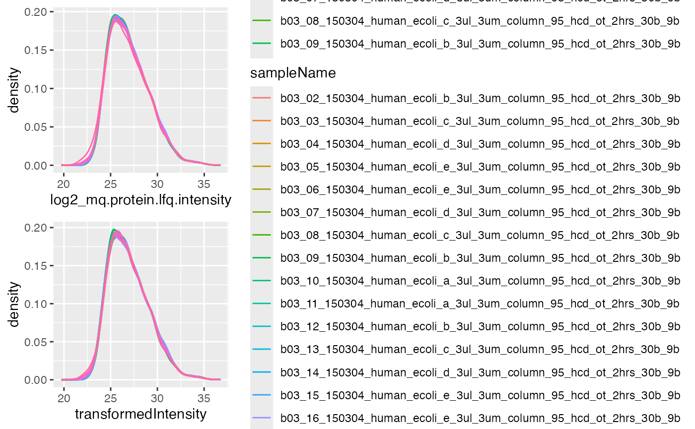
Distribution of intensites before (left panel) and after (right panel) robscaling.
To use proDA, we need to create an
SummarizedExperiment, which is easily to be done using the
to_wide function of prolfqua.
library(SummarizedExperiment)
wide <- lfqtrans$to_wide(as.matrix = TRUE)
library(SummarizedExperiment)
ann <- data.frame(wide$annotation)
rownames(ann) <- wide$annotation$sampleName

se <- SummarizedExperiment(SimpleList(LFQ=wide$data), colData = ann)
Defining Contrasts and computing group comparisons
As usual, two steps are required, first fit the models, then comptue the contrasts.
fit <- proDA::proDA(se, design = ~ dilution. - 1,data_is_log_transformed = TRUE)
contr <- list()
contr[["dilution_(9/7.5)_1.2"]] <- data.frame(
  contrast = "dilution_(9/7.5)_1.2",
  proDA::test_diff(fit, contrast = "dilution.e - dilution.d"))
contr[["dilution_(7.5/6)_1.25"]] <- data.frame(
  contrast = "dilution_(7.5/6)_1.25",
  proDA::test_diff(fit, contrast = "dilution.d - dilution.c"))
contr[["dilution_(6/4.5)_1.3(3)"]] <- data.frame(
  contrast = "dilution_(6/4.5)_1.3(3)",
  proDA::test_diff(fit, contrast = "dilution.c - dilution.b"))
contr[["dilution_(4.5/3)_1.5"]] <- data.frame(
  contrast = "dilution_(4.5/3)_1.5",
  proDA::test_diff(fit, contrast = "dilution.b - dilution.a" ))

bb <- dplyr::bind_rows(contr)
Benchmarking
## [1] 4235
ttd <- prolfqua::ionstar_bench_preprocess( bb , idcol = "name" )
benchmark_proDA <- prolfqua::make_benchmark(ttd$data,
                                            contrast = "contrast",
                                            avgInt = "avg_abundance",
                                            toscale = c("pval"),
                                            fcestimate = "diff",
                                            benchmark = list(
                                              list(score = "diff", desc = TRUE),
                                              list(score = "t_statistic", desc = TRUE),
                                              list(score = "scaled.pval", desc = TRUE)
                                            ),
                                            model_description = "proDA_lfqInt",
                                            model_name = "proDA_lfqInt",
                                            FDRvsFDP = list(list(score = "adj_pval", desc = FALSE))
                                            , hierarchy = c("name"), summarizeNA = "t_statistic"
)

sum(benchmark_proDA$smc$summary$name)
## [1] 4235
sumarry <- benchmark_proDA$smc$summary
prolfqua::table_facade(sumarry, caption = "nr of proteins with 0, 1, 2, 3 missing contrasts.")| nr_missing | name |
|---|---|
| 0 | 4229 |
| 4 | 6 |
res <- benchmark_proDA$pAUC_summaries()
knitr::kable(res$ftable$content,caption = res$ftable$caption)| contrast | what | AUC | pAUC_10 | pAUC_20 |
|---|---|---|---|---|
| all | diff | 87.09292 | 49.73182 | 65.37813 |
| all | scaled.pval | 88.72047 | 65.75239 | 70.89986 |
| all | t_statistic | 88.72047 | 65.75239 | 70.89986 |
| dilution_(4.5/3)_1.5 | diff | 86.63464 | 42.39732 | 58.71807 |
| dilution_(4.5/3)_1.5 | scaled.pval | 87.89786 | 63.23296 | 67.08638 |
| dilution_(4.5/3)_1.5 | t_statistic | 87.89786 | 63.23296 | 67.08638 |
| dilution_(6/4.5)_1.3(3) | diff | 84.53780 | 51.30018 | 64.70222 |
| dilution_(6/4.5)_1.3(3) | scaled.pval | 87.54385 | 64.41084 | 69.19538 |
| dilution_(6/4.5)_1.3(3) | t_statistic | 87.54385 | 64.41084 | 69.19538 |
| dilution_(7.5/6)_1.25 | diff | 87.02231 | 48.36063 | 64.93901 |
| dilution_(7.5/6)_1.25 | scaled.pval | 88.66198 | 64.50954 | 70.58000 |
| dilution_(7.5/6)_1.25 | t_statistic | 88.66198 | 64.50954 | 70.58000 |
| dilution_(9/7.5)_1.2 | diff | 89.94294 | 58.26490 | 73.48897 |
| dilution_(9/7.5)_1.2 | scaled.pval | 90.79189 | 70.18542 | 76.43784 |
| dilution_(9/7.5)_1.2 | t_statistic | 90.79189 | 70.18542 | 76.43784 |
res$barp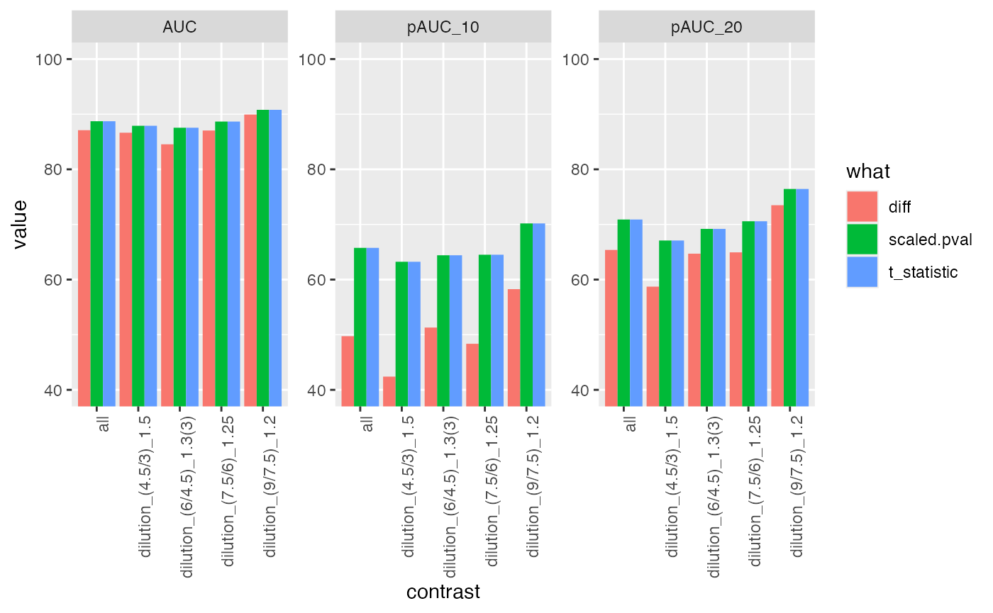
ROC curves
#res$ftable
benchmark_proDA$plot_ROC(xlim = 0.2)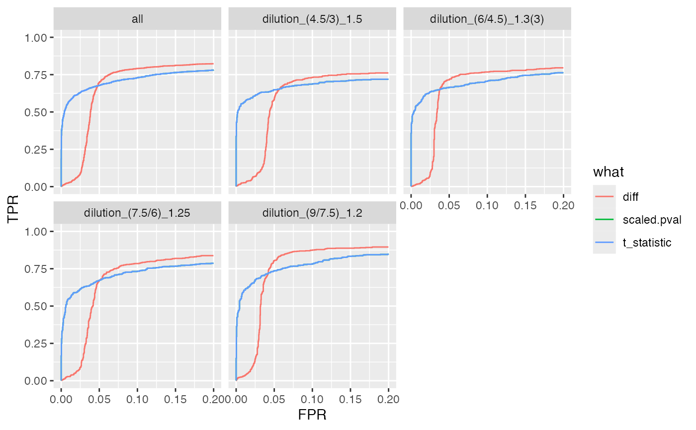
plot ROC curves
benchmark_proDA$plot_FDRvsFDP()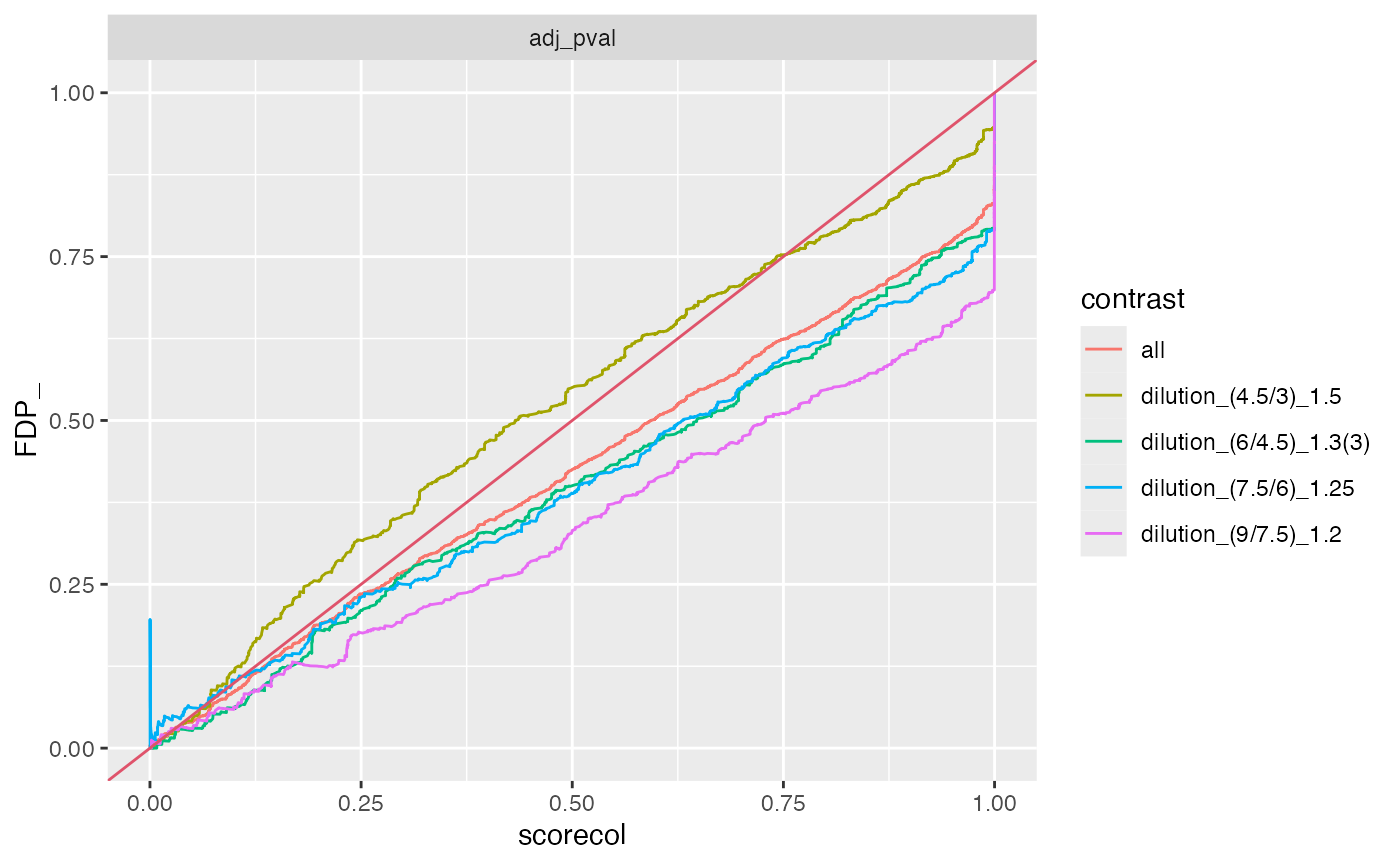
plot FDR vs FDP
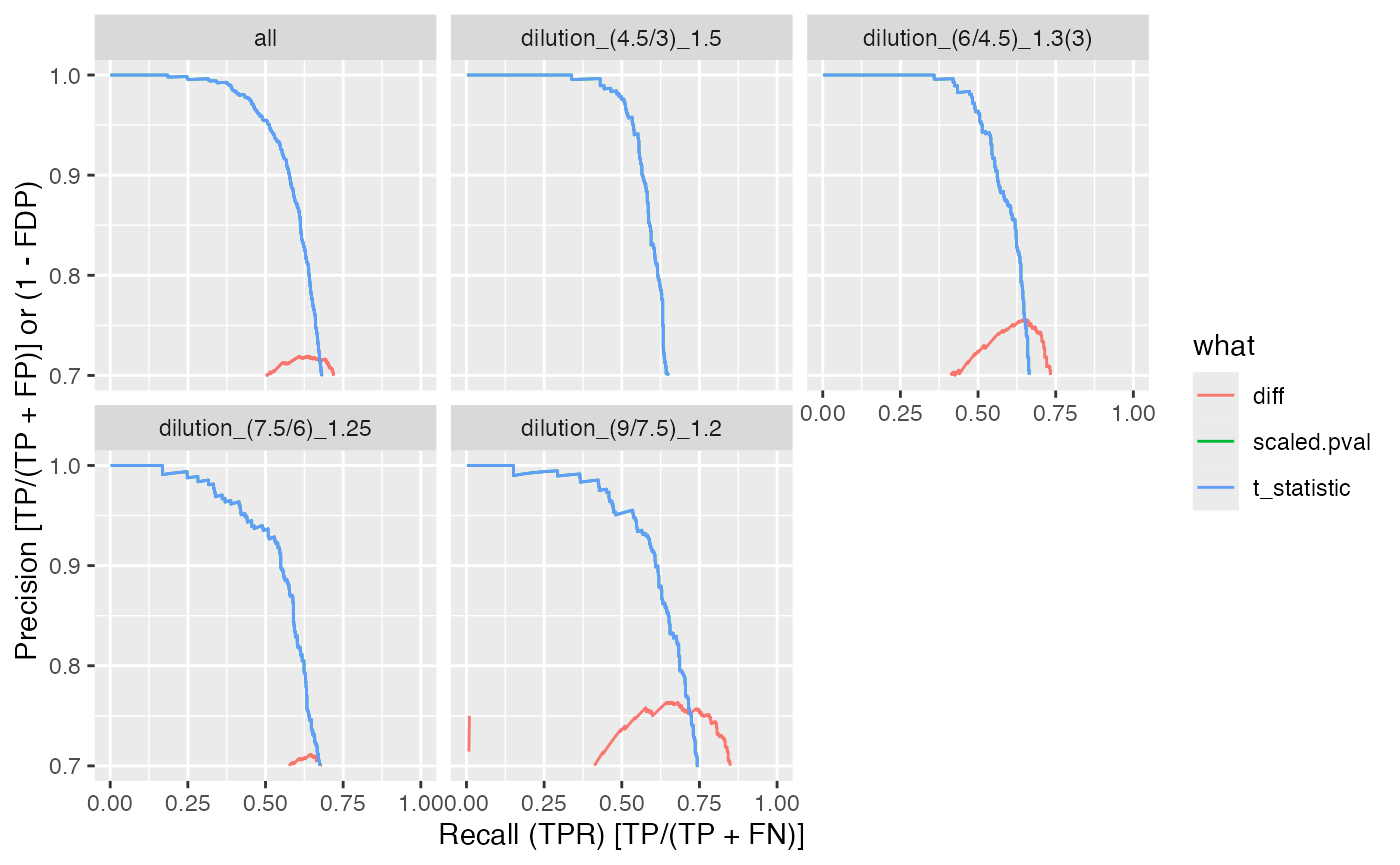
benchmark_proDA$plot_precision_recall()