Benchmarking robust linear model using the Ionstar Dataset

Please download and install the prolfquadata package from github

conflicted::conflict_prefer("filter", "dplyr")

Decide if you work with all data or for speedup with subset of data:

SUBSET <- FALSE
SUBSETNORM <- TRUE
SAVE <- TRUE

We start by loading the IonStar dataset and the annotation from the prolfquadata package. The method add_annotation adds the annotation to the data.

datadir <- file.path(find.package("prolfquadata") , "quantdata")
inputMQfile <-  file.path(datadir,
                          "MAXQuant_IonStar2018_PXD003881.zip")
inputAnnotation <- file.path(datadir, "annotation_Ionstar2018_PXD003881.xlsx")
mqdata <- list()

mqdata$data <- prolfquapp::tidyMQ_Peptides(inputMQfile)
length(unique(mqdata$data$proteins))

## [1] 5295

mqdata$config <- prolfqua::create_config_MQ_peptide()


annotation <- readxl::read_xlsx(inputAnnotation)
res <- prolfquapp::add_annotation(
  mqdata$data,
  annotation,
  fileName = "raw.file"
)

The setup_analysis asserts that all columns specified in the configruation are present in the data. For more details about the prolfqua configuration see the vignette “Creating Configurations”.

mqdata$config$table$factors[["dilution."]] = "sample"
mqdata$config$table$factors[["run_Id"]] = "run_ID"
mqdata$config$table$factorDepth <- 1
mqdata$data <- prolfqua::setup_analysis(res, mqdata$config)

Data normalization

First we remove all contaminant, decoy proteins from the list, than we remove 0 intensity values, then filter for 2 peptides per protein.

lfqdata <- prolfqua::LFQData$new(mqdata$data, mqdata$config)
lfqdata$data <- lfqdata$data |> dplyr::filter(!grepl("^REV__|^CON__", protein_Id)) 
sr <- lfqdata$get_Summariser()
lfqdata$remove_small_intensities()
sr <- lfqdata$get_Summariser()
sr$hierarchy_counts()

## # A tibble: 1 × 3
##   isotope protein_Id peptide_Id
##   <chr>        <int>      <int>
## 1 light         4777      30478

We will normalize the data using the ‘LFQTransformer’ class. Since we know that the Human proteins are the Matrix in the experiment we will normalize the data using HUMAN proteins only. To this task we subset the dataset by filtering for HUMAN proteins only and then use the LFQDataTransformer to normalize the data.

tr <- lfqdata$get_Transformer()
subset_h <- lfqdata$get_copy()
subset_h$data <- subset_h$data |> dplyr::filter(grepl("HUMAN", protein_Id))
subset_h <- subset_h$get_Transformer()$log2()$lfq
lfqdataNormalized <- tr$log2()$robscale_subset(lfqsubset = subset_h,  preserveMean = FALSE )$lfq

The figures below show the intensity distribution before and after normalization.

before <- lfqdata$get_Plotter()
before$intensity_distribution_density()

after <- lfqdataNormalized$get_Plotter()
after$intensity_distribution_density()

Create a sample of N proteins to speed up computations of models and contrasts.

if (SUBSET) {
  N <- 200
  mqdataSubset <- lfqdata$get_sample(size = N, seed = 2020)
  lfqNormSubset <- lfqdataNormalized$get_sample(size = N, seed = 2020)
  lfqNormSubset$hierarchy_counts()
} else {
  mqdataSubset <- lfqdata$get_copy()  
  lfqNormSubset <- lfqdataNormalized$clone()
  lfqNormSubset$hierarchy_counts()
}

## # A tibble: 1 × 3
##   isotope protein_Id peptide_Id
##   <chr>        <int>      <int>
## 1 light         4777      30478

Fitting a robust linear model to peptide abundances

df.residual.rlm <- function(object, ...) {
  return( sum(object$w) - object$rank)
}


sigma.rlm <- function(object, ...) {
  sqrt(sqrt(sum(object$w * object$resid^2) / (sum(object$w) - object$rank)))
}


rlmmodel <- "~ dilution."
rlmmodel <- paste0(lfqNormSubset$config$table$get_response() , rlmmodel)
lfqNormSubset$config$table$hierarchyDepth <- 1

modelFunction <- prolfqua::strategy_rlm( rlmmodel, model_name = "Model")

mod_rlm_ProtLevel <- prolfqua::build_model(lfqNormSubset$data, modelFunction)
mod_rlm_ProtLevel$get_anova()

## # A tibble: 4,639 × 10
##    protein_Id      isSingular nrcoef factor    Df Sum.Sq Mean.Sq F.value p.value
##    <chr>           <lgl>       <int> <chr>  <dbl>  <dbl>   <dbl>   <dbl>   <dbl>
##  1 sp|A0AVT1|UBA6… FALSE           5 dilut…     4 0.533   0.133   0.414    0.798
##  2 sp|A0FGR8|ESYT… FALSE           5 dilut…     4 0.0711  0.0178  0.0213   0.999
##  3 sp|A0MZ66|SHOT… FALSE           5 dilut…     4 0.581   0.145   0.224    0.925
##  4 sp|A1L0T0|ILVB… FALSE           5 dilut…     4 0.386   0.0965  0.246    0.910
##  5 sp|A1X283|SPD2… FALSE           5 dilut…     4 0.410   0.102   0.522    0.720
##  6 sp|A2RRP1|NBAS… FALSE           5 dilut…     4 0.118   0.0296  0.314    0.867
##  7 sp|A3KN83|SBNO… FALSE           5 dilut…     4 1.27    0.317   0.791    0.539
##  8 sp|A4D1E9|GTPB… FALSE           5 dilut…     4 0.825   0.206   0.693    0.599
##  9 sp|A5PLL7|TM18… FALSE           5 dilut…     4 0.834   0.208   0.115    0.976
## 10 sp|A5YKK6|CNOT… FALSE           5 dilut…     4 0.774   0.194   0.244    0.913
## # ℹ 4,629 more rows
## # ℹ 1 more variable: FDR <dbl>

mod_rlm_ProtLevel$anova_histogram()$plot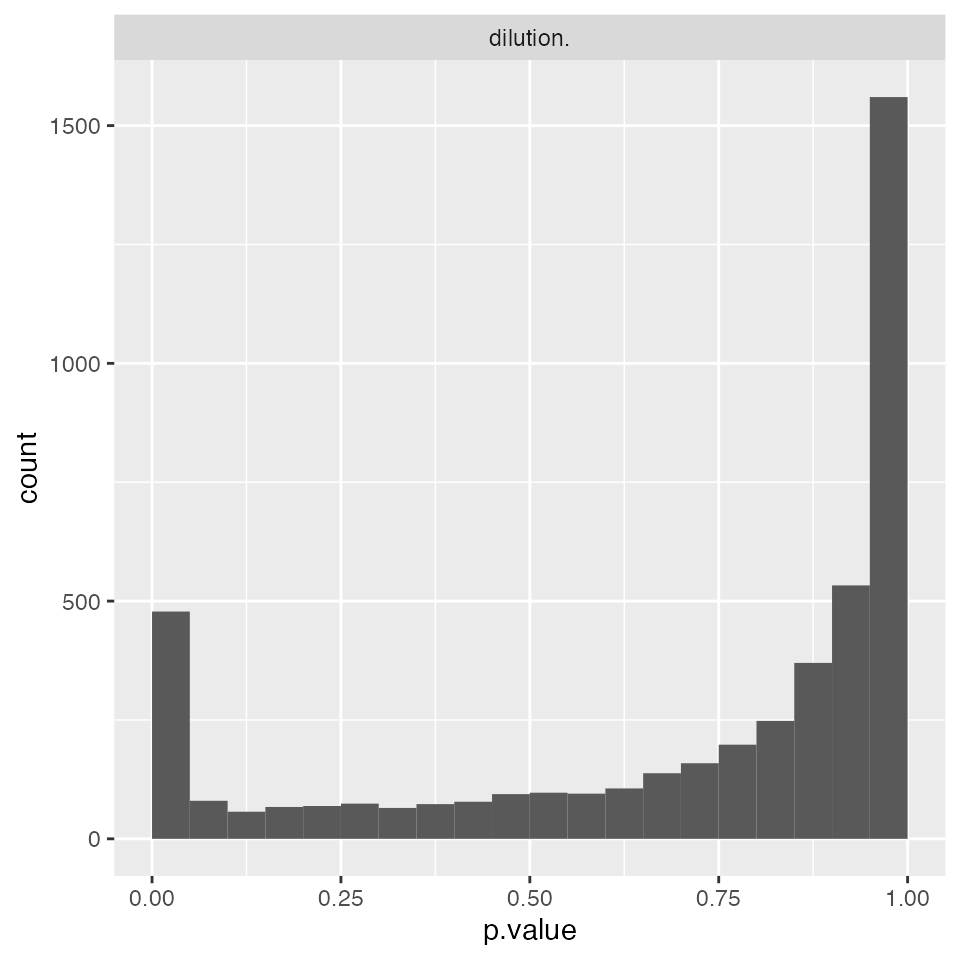

Computing Contrasts

Once models are fitted contrasts can be computed. The R code below defines all possible contrasts among conditions for the ionstar dataset.

DEBUG <- FALSE

Contrasts <- c(
  "dilution_(9/3)_3" =   "dilution.e - dilution.a",
  "dilution_(9/4.5)_2" =   "dilution.e - dilution.b",
  "dilution_(9/6)_1.5" =   "dilution.e - dilution.c",
  "dilution_(9/7.5)_1.2" =   "dilution.e - dilution.d",
  
  "dilution_(7.5/3)_2.5" =   "dilution.d - dilution.a",
  "dilution_(7.5/4.5)_1.6(6)" =   "dilution.d - dilution.b",
  "dilution_(7.5/6)_1.25" =   "dilution.d - dilution.c",
  
  "dilution_(6/3)_2" =   "dilution.c - dilution.a",
  "dilution_(6/4.5)_1.3(3)" =   "dilution.c - dilution.b",
  
  "dilution_(4.5/3)_1.5" =   "dilution.b - dilution.a"
)


tt <- Reduce(rbind, strsplit(names(Contrasts),split = "_"))
tt <- data.frame(tt)[,2:3]
colnames(tt) <- c("ratio" , "expected fold-change")
tt <- tibble::add_column(tt, contrast =  Contrasts, .before = 1)
prolfqua::table_facade(
  tt,
  caption = "All possible Contrasts given 5 E. coli dilutions of the Ionstar Dataset", digits = 1)

All possible Contrasts given 5 E. coli dilutions of the Ionstar Dataset
	contrast	ratio	expected fold-change
init	dilution.e - dilution.a	(9/3)	3
X	dilution.e - dilution.b	(9/4.5)	2
X.1	dilution.e - dilution.c	(9/6)	1.5
X.2	dilution.e - dilution.d	(9/7.5)	1.2
X.3	dilution.d - dilution.a	(7.5/3)	2.5
X.4	dilution.d - dilution.b	(7.5/4.5)	1.6(6)
X.5	dilution.d - dilution.c	(7.5/6)	1.25
X.6	dilution.c - dilution.a	(6/3)	2
X.7	dilution.c - dilution.b	(6/4.5)	1.3(3)
X.8	dilution.b - dilution.a	(4.5/3)	1.5

relevantContrasts <- c("dilution_(9/7.5)_1.2",
                       "dilution_(7.5/6)_1.25",
                       "dilution_(6/4.5)_1.3(3)",
                       "dilution_(4.5/3)_1.5" )

tt <- Reduce(rbind, strsplit(relevantContrasts,split = "_"))
tt <- data.frame(tt)[,2:3]
colnames(tt) <- c("ratio" , "expected fold-change")
tt <- tibble::add_column(tt, contrast =  Contrasts[names(Contrasts) %in% relevantContrasts], .before = 1)
prolfqua::table_facade(tt, caption = "Contrasts used for benchmark.", digits = 1)

Contrasts used for benchmark.
	contrast	ratio	expected fold-change
init	dilution.e - dilution.d	(9/7.5)	1.2
X	dilution.d - dilution.c	(7.5/6)	1.25
X.1	dilution.c - dilution.b	(6/4.5)	1.3(3)
X.2	dilution.b - dilution.a	(4.5/3)	1.5

relevantContrasts <- Contrasts[names(Contrasts) %in% relevantContrasts]

Contrasts from robust linear model

Adding Moderation to RLM model

contrProtRLMModerated <- prolfqua::ContrastsModerated$new(contrProt_RLM)
contrProtRLMModerated$get_Plotter()$volcano()$FDR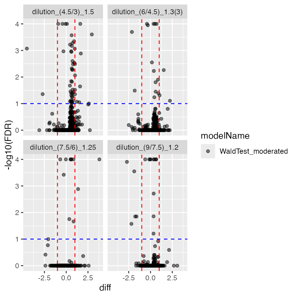

contrProtRLMModerated$get_contrasts()$protein_Id |> unique() |> length()

## [1] 4731

ttd <- prolfqua::ionstar_bench_preprocess(contrProtRLMModerated$get_contrasts())
benchmark_ProtRLMModerated <- prolfqua::make_benchmark(
    ttd$data,
    model_description = "med. polish and rlm moderated",
    model_name = "prolfqua_rlm_mod")

prolfqua::table_facade(
  benchmark_ProtRLMModerated$smc$summary,
  caption = "Nr of proteins with Nr of not estimated contrasts.",
  digits = 1)

Nr of proteins with Nr of not estimated contrasts.
nr_missing	protein_Id
0	4479
1	87
2	73
3	33
4	59

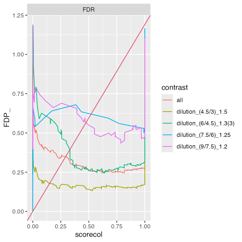
benchmark_ProtRLMModerated$plot_ROC(xlim = 1)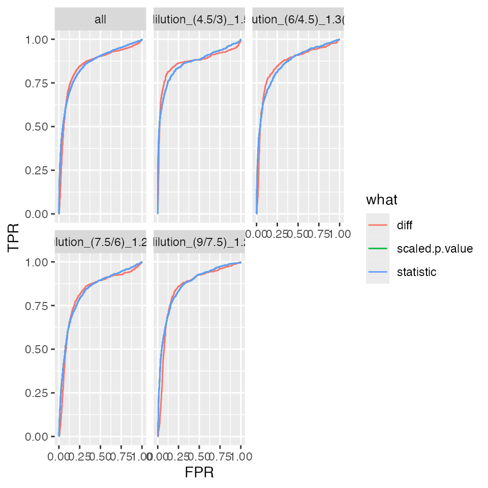

benchmark_ProtRLMModerated$plot_FDRvsFDP()

Witold E Wolski

2024-06-29

Data normalization

Fitting a robust linear model to peptide abundances

Computing Contrasts

Contrasts from robust linear model

Adding Moderation to RLM model