Benchmarking normalization, aggregation and models using the Ionstar Dataset
Witold Wolski
2026-02-25
Source:vignettes/BenchmarkingIonstarData.Rmd
BenchmarkingIonstarData.RmdPlease download and install the prolfquadata package
from github
conflicted::conflict_prefer("filter", "dplyr")Decide if you work with all data or for speedup with subset of data:
SUBSET <- FALSE
SUBSETNORM <- TRUE
SAVE <- TRUE
We start by loading the IonStar dataset and the annotation from the
prolfquadata package.
datadir <- file.path(find.package("prolfquadata") , "quantdata")
inputMQfile <-  file.path(datadir,
                          "MAXQuant_IonStar2018_PXD003881.zip")
inputAnnotation <- file.path(datadir, "annotation_Ionstar2018_PXD003881.xlsx")
mqdata <- list()

mqdata$data <- prolfquapp::tidyMQ_Peptides(inputMQfile)
length(unique(mqdata$data$proteins))
## [1] 5295
mqdata$config <- prolfqua::create_config_MQ_peptide()


annotation <- readxl::read_xlsx(inputAnnotation)
res <- dplyr::inner_join(
  mqdata$data,
  annotation,
  by = "raw.file"
)
The setup_analysis asserts that all columns specified in
the configruation are present in the data. For more details about the
prolfqua configuration see the vignette “Creating
Configurations”.
mqdata$config$table$factors[["dilution."]] = "sample"
mqdata$config$table$factors[["run_Id"]] = "run_ID"
mqdata$config$table$factorDepth <- 1
mqdata$data <- prolfqua::setup_analysis(res, mqdata$config)
Data filtering and normalization
First we remove all contaminant, decoy proteins from the list, than we remove 0 intensity values, then filter for 2 peptides per protein.
lfqdata <- prolfqua::LFQData$new(mqdata$data, mqdata$config)Filter the data for small intensities (maxquant reports missing values as 0) and for two peptides per protein.
lfqdata$data <- lfqdata$data |> dplyr::filter(!grepl("^REV__|^CON__", protein_Id))
lfqdata$filter_proteins_by_peptide_count()
lfqdata$remove_small_intensities()
lfqdata$hierarchy_counts()
## # A tibble: 1 × 3
## isotope protein_Id peptide_Id
## <chr> <int> <int>
## 1 light 4178 29879We will normalize the data using the ‘LFQTransformer’ class. Since we
know that the Human proteins are the Matrix in the experiment we will
normalize the data using HUMAN proteins only. To this task we subset the
dataset by filtering for HUMAN proteins only and then use the
LFQDataTransformer to normalize the data.
tr <- lfqdata$get_Transformer()
subset_h <- lfqdata$get_copy()
subset_h$data <- subset_h$data |> dplyr::filter(grepl("HUMAN", protein_Id))
subset_h <- subset_h$get_Transformer()$log2()$lfq
lfqdataNormalized <- tr$log2()$robscale_subset(lfqsubset = subset_h,  preserveMean = FALSE )$lfq
The figures below show the intensity distribution before and after normalization.
before <- lfqdata$get_Plotter()
before$intensity_distribution_density()
after <- lfqdataNormalized$get_Plotter()
after$intensity_distribution_density()
Create a sample of N proteins to speed up computations of models and contrasts.
if (SUBSET) {
  N <- 200
  mqdataSubset <- lfqdata$get_sample(size = N, seed = 2020)
  lfqNormSubset <- lfqdataNormalized$get_sample(size = N, seed = 2020)
  lfqNormSubset$hierarchy_counts()
} else {
  mqdataSubset <- lfqdata$get_copy()
  lfqNormSubset <- lfqdataNormalized$clone()
  lfqNormSubset$hierarchy_counts()
}
## # A tibble: 1 × 3
## isotope protein_Id peptide_Id
## <chr> <int> <int>
## 1 light 4178 29879Inferring Protein abundances from Peptide abundances
We will be using the LFQDataAggregator class. To
estimate protein abundances using Tukey’s median polish we need to use
log2 transformed peptide abundances
lfqNormSubset$config$table$get_response()## [1] "transformed_abundance"
pl <- lfqNormSubset$get_Plotter()
pl$intensity_distribution_density()
lfqAggMedpol <- lfqNormSubset$get_Aggregator()
lfqAggMedpol$medpolish()
The figure below shows the the peptide abundances used for estimation and the protein abundance estimates (black line).
xx <- lfqAggMedpol$plot()
gridExtra::grid.arrange(grobs =  xx$plots[1:3])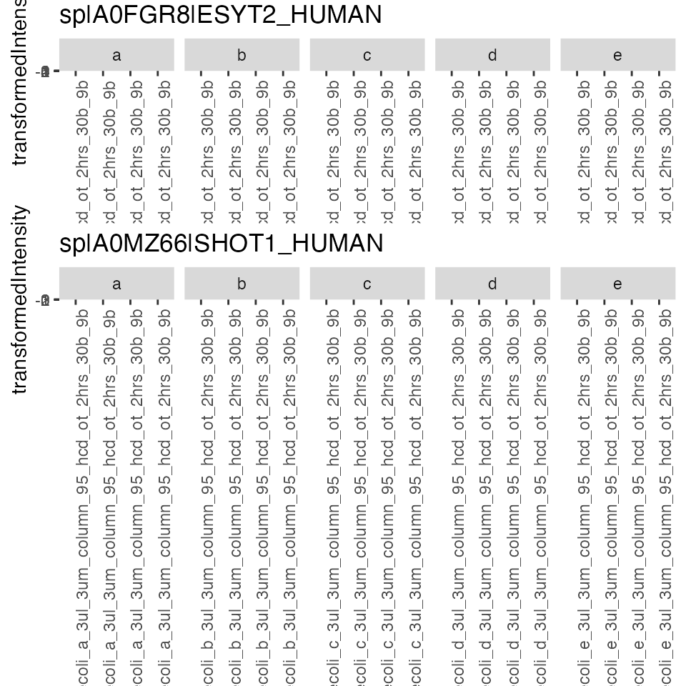
We can also estimate the protein abundances by adding the abundances of the top N most abundant peptides. In this case we are using the untransformed peptide abudances.
lfqAggregator <- lfqdata$get_Aggregator()
lfqAggregator$mean_topN()
topN <- lfqAggregator$plot()
topN$plots[[1]]
Model Fitting
We will be fitting tree models to the data:
- The first model is a linear model as implemented by the R function
lmfitted to protein abundances inferred from peptide abundances using the LFQAggregator. - The second model is mixed effects model implemented in the R
function
lmerfitted to peptide abundances, where we model the peptide measurements as repeated measurements of the protein. - The third model again is a linear model but fitted to peptide abundances. By this we obtain for each peptide a linear model can compute contrasts and then can aggregate them using the ROPECA method.
Fitting a linear model to the protein abundances
protLFQ <- lfqAggMedpol$lfq_agg
sr <- protLFQ$get_Summariser()
sr$hierarchy_counts()
## # A tibble: 1 × 2
## isotope protein_Id
## <chr> <int>
## 1 light 4178
lmmodel <- "~ dilution."
lmmodel <- paste0(protLFQ$config$table$get_response() , lmmodel)

lfqNormSubset$config$table$hierarchyDepth <- 1
modelFunction <- prolfqua::strategy_lm( lmmodel, model_name = "Model")

modLinearProt <- prolfqua::build_model(protLFQ$data, modelFunction)
modLinearProt$anova_histogram()$plot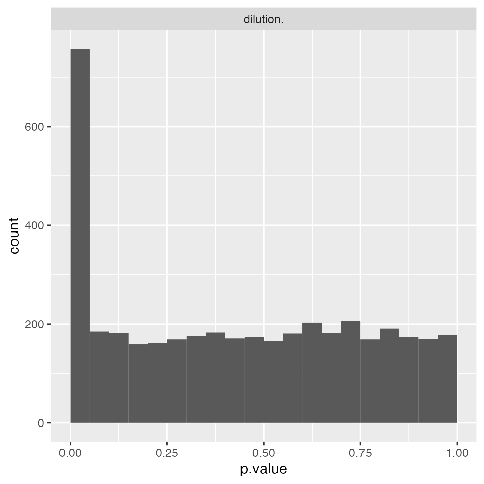
Fitting a mixed effects model to peptide abundances
lmmodel <- "~ dilution. + (1|peptide_Id) + (1|sampleName)"
lmmodel <- paste0(lfqNormSubset$config$table$get_response() , lmmodel)
lfqNormSubset$config$table$hierarchyDepth <- 1
modelFunction <- prolfqua::strategy_lmer( lmmodel, model_name = "Model")
modMixedProtLevel <- prolfqua::build_model(lfqNormSubset$data, modelFunction)
modMixedProtLevel$anova_histogram()$plot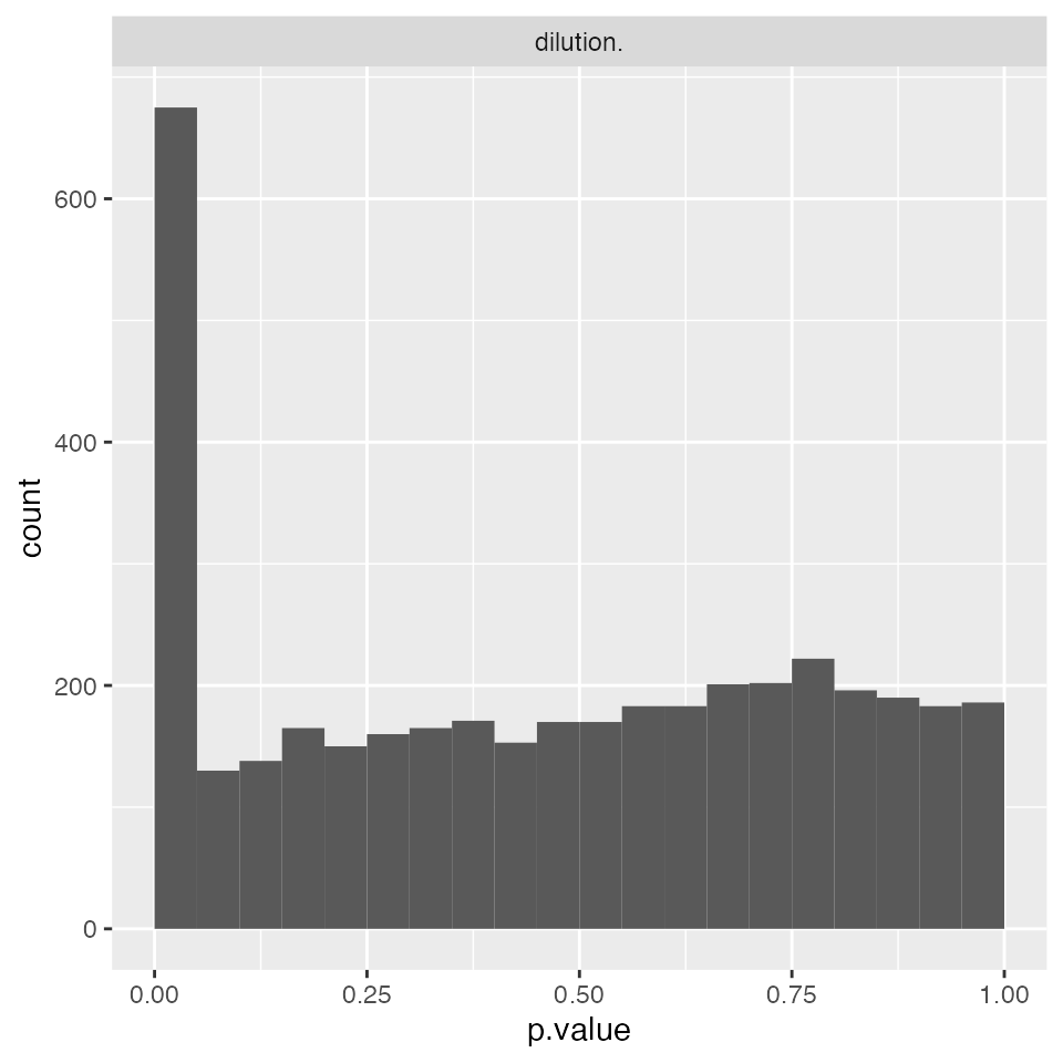
Fitting peptide level models
lmmodel <- "~ dilution."

lfqNormSubset$config$table$hierarchyDepth
## [1] 1
lfqNormSubset$config$table$hierarchyDepth <- 2

lmmodel <- paste0(lfqNormSubset$config$table$get_response() , lmmodel)

modelFunction <- prolfqua::strategy_lm( lmmodel, model_name = "Model")
modLMPepLevel <- prolfqua::build_model(lfqNormSubset$data,
                                       modelFunction,
                                       subject_Id = lfqNormSubset$subject_Id())
modLMPepLevel$anova_histogram()$plot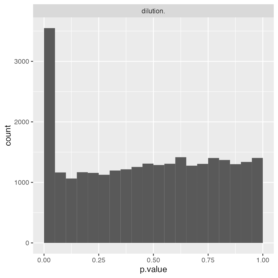
Computing Contrasts
Once models are fitted contrasts can be computed. The R code below defines all possible contrasts among conditions for the ionstar dataset.
DEBUG <- FALSE

Contrasts <- c(
  "dilution_(9/3)_3" =   "dilution.e - dilution.a",
  "dilution_(9/4.5)_2" =   "dilution.e - dilution.b",
  "dilution_(9/6)_1.5" =   "dilution.e - dilution.c",
  "dilution_(9/7.5)_1.2" =   "dilution.e - dilution.d",

  "dilution_(7.5/3)_2.5" =   "dilution.d - dilution.a",
  "dilution_(7.5/4.5)_1.6(6)" =   "dilution.d - dilution.b",
  "dilution_(7.5/6)_1.25" =   "dilution.d - dilution.c",

  "dilution_(6/3)_2" =   "dilution.c - dilution.a",
  "dilution_(6/4.5)_1.3(3)" =   "dilution.c - dilution.b",

  "dilution_(4.5/3)_1.5" =   "dilution.b - dilution.a"
)


tt <- Reduce(rbind, strsplit(names(Contrasts),split = "_"))
tt <- data.frame(tt)[,2:3]
colnames(tt) <- c("ratio" , "expected fold-change")
tt <- tibble::add_column(tt, contrast =  Contrasts, .before = 1)
prolfqua::table_facade(
  tt,
caption = "All possible Contrasts given 5 E. coli dilutions of the Ionstar Dataset", digits = 1)| contrast | ratio | expected fold-change |
|---|---|---|
| dilution.e - dilution.a | (9/3) | 3 |
| dilution.e - dilution.b | (9/4.5) | 2 |
| dilution.e - dilution.c | (9/6) | 1.5 |
| dilution.e - dilution.d | (9/7.5) | 1.2 |
| dilution.d - dilution.a | (7.5/3) | 2.5 |
| dilution.d - dilution.b | (7.5/4.5) | 1.6(6) |
| dilution.d - dilution.c | (7.5/6) | 1.25 |
| dilution.c - dilution.a | (6/3) | 2 |
| dilution.c - dilution.b | (6/4.5) | 1.3(3) |
| dilution.b - dilution.a | (4.5/3) | 1.5 |
relevantContrasts <- c("dilution_(9/7.5)_1.2",
                       "dilution_(7.5/6)_1.25",
                       "dilution_(6/4.5)_1.3(3)",
                       "dilution_(4.5/3)_1.5" )

tt <- Reduce(rbind, strsplit(relevantContrasts,split = "_"))
tt <- data.frame(tt)[,2:3]
colnames(tt) <- c("ratio" , "expected fold-change")
tt <- tibble::add_column(tt, contrast =  Contrasts[names(Contrasts) %in% relevantContrasts], .before = 1)
prolfqua::table_facade(tt, caption = "Contrasts used for benchmark.", digits = 1)| contrast | ratio | expected fold-change |
|---|---|---|
| dilution.e - dilution.d | (9/7.5) | 1.2 |
| dilution.d - dilution.c | (7.5/6) | 1.25 |
| dilution.c - dilution.b | (6/4.5) | 1.3(3) |
| dilution.b - dilution.a | (4.5/3) | 1.5 |
There are, as of today, four contrasts classes in the package prolfqua:
- ‘ContrastsSimpleImputed’ : contrast computation with imputation of fold changes and t-statistic estimation using pooled variances.
- ‘Contrasts’ : uses Wald test,
- ‘ContrastsModerated’ : applies variance moderation,
- ‘ContrastsROPECA’ implements difference and p-value aggregation
Contrasts with Imputation
In order to estimate differences (fold-changes), statistics and p-values of proteins for which linear models could not be fitted because of an excess of missing measurements, the following procedure is applied. The mean abundance of a protein in a condition is computed. For the proteins with no observation in a condition, we infer their abundances by using the mean protein abundances observed only in one sample per group. The standard deviation of the protein is estimated using the pooled variances of the condition where the variance could be estimated.
contrImp <- prolfqua::ContrastsMissing$new(
  protLFQ,
  relevantContrasts)

bb <- contrImp$get_contrasts()

plc <- contrImp$get_Plotter()
plc$volcano()$FDR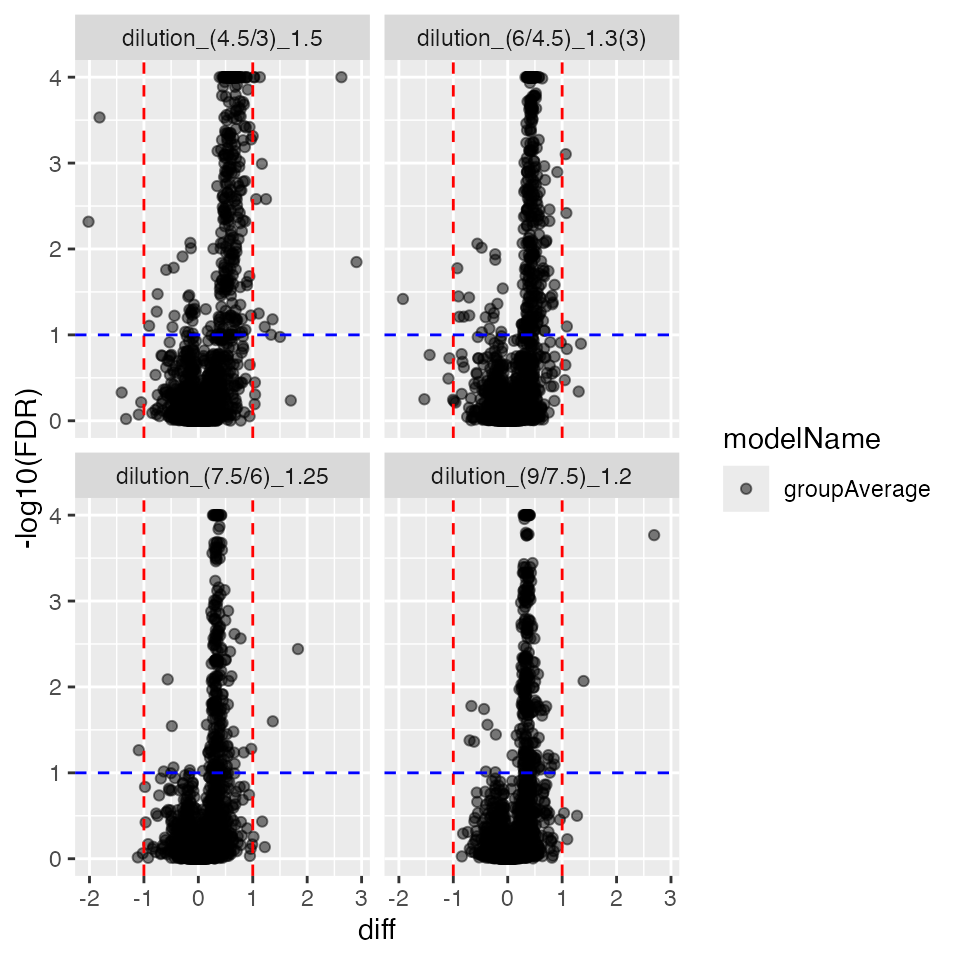
plc$ma_plot()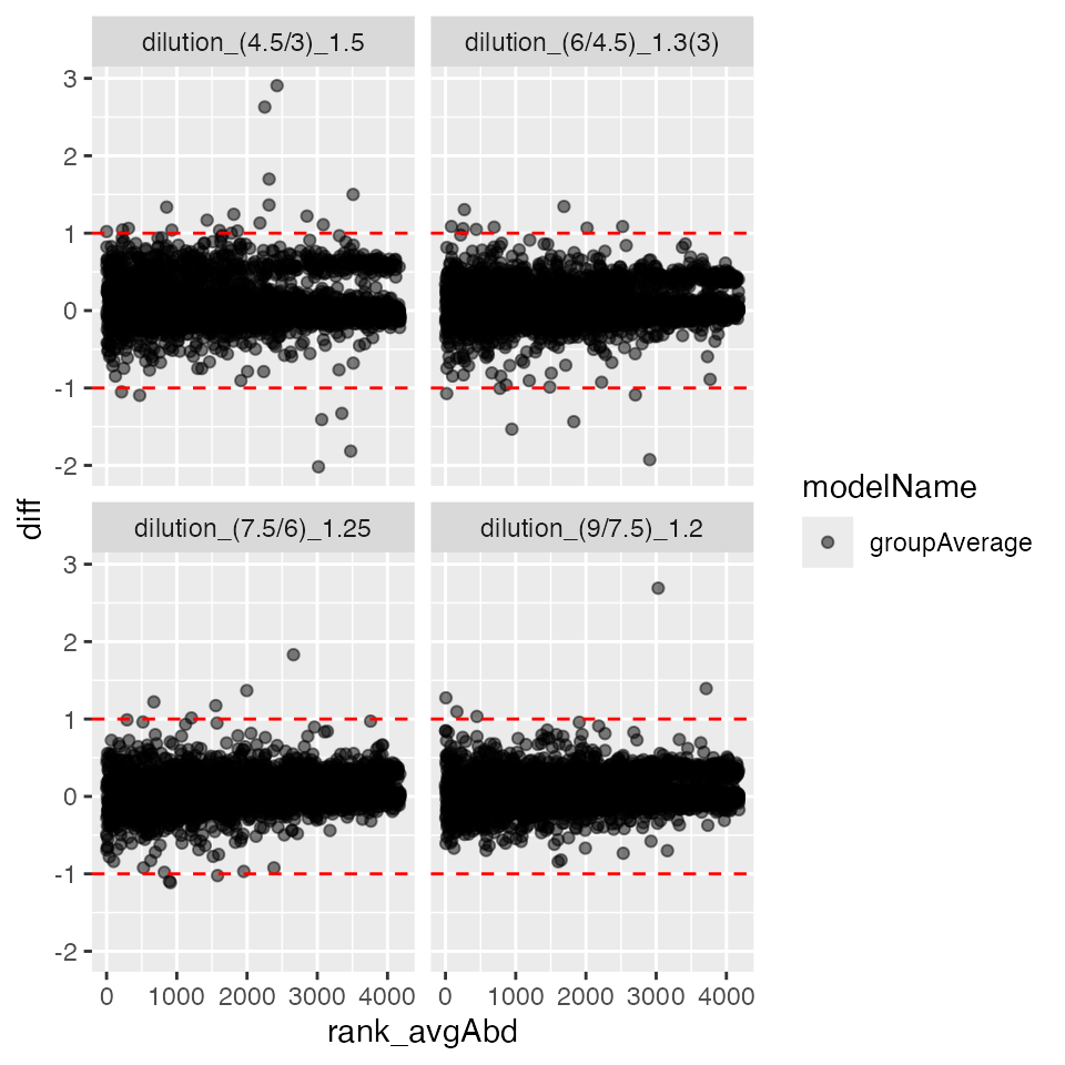
plc$histogram()$p.value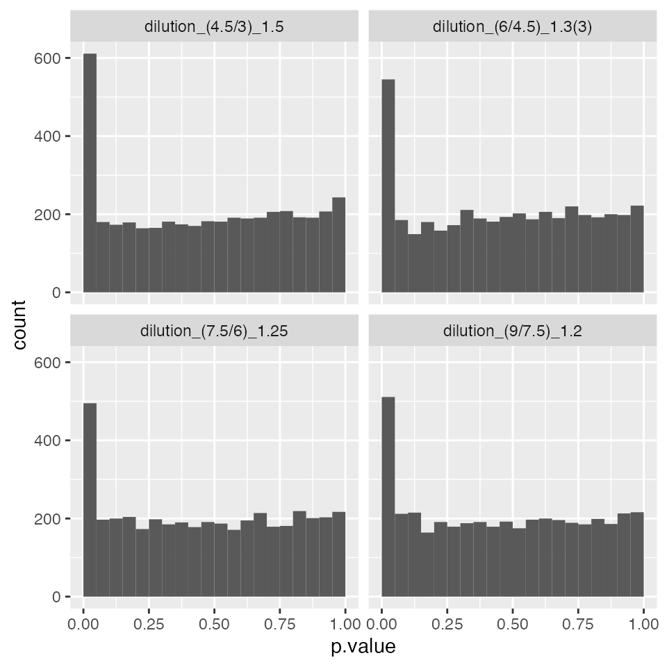
allContrasts <- list()
allContrasts$imputation <- contrImp$get_contrasts()
ttd <- prolfqua::ionstar_bench_preprocess(contrImp$get_contrasts())

benchmark_missing <- prolfqua::make_benchmark(
    ttd$data,
    model_description = "med. polish and missingness modelling",
    model_name = "prolfqua_missing",
    FDRvsFDP = list(list(score = "FDR", desc = FALSE))
)

benchmark_missing$plot_ROC(xlim = 0.1)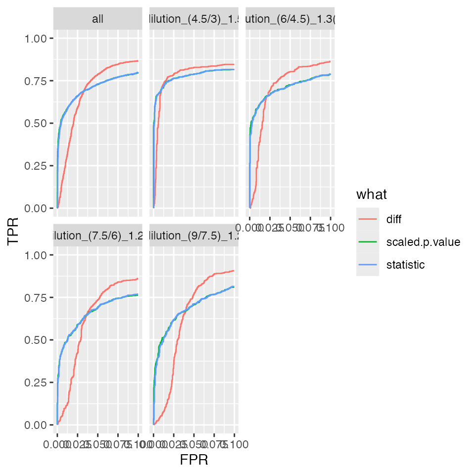
benchmark_missing$plot_FDRvsFDP()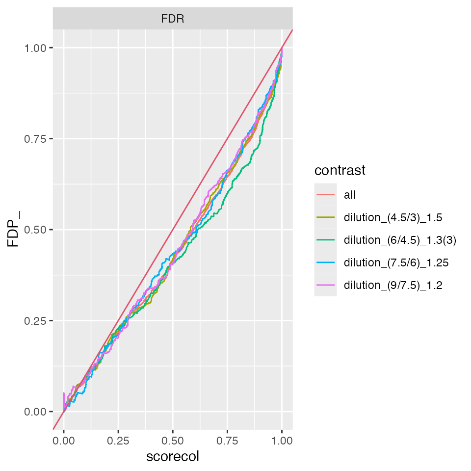
prolfqua::table_facade(benchmark_missing$smc$summary, caption = "Nr of proteins with Nr of not estimated contrasts.", digits = 1)| nr_missing | protein_Id |
|---|---|
| 0 | 4178 |
bb <- benchmark_missing$pAUC_summaries()
bb$barp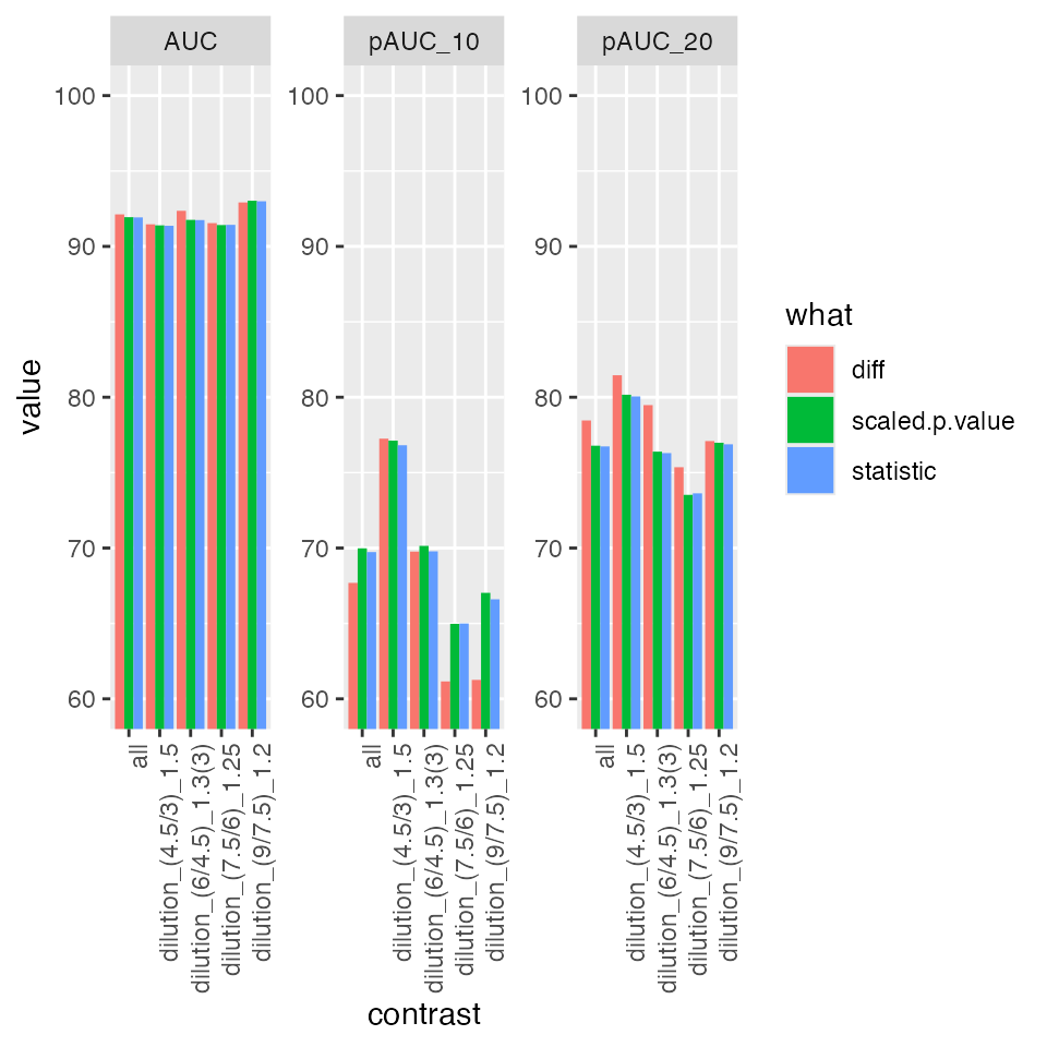
Summary of partial area under the ROC curve.
prolfqua::table_facade(bb$ftable$content, caption = bb$ftable$caption, digits = 1)| contrast | what | AUC | pAUC_10 | pAUC_20 |
|---|---|---|---|---|
| all | diff | 92.1 | 67.7 | 78.5 |
| all | scaled.p.value | 91.9 | 70.0 | 76.8 |
| all | statistic | 91.9 | 69.7 | 76.7 |
| dilution_(4.5/3)_1.5 | diff | 91.5 | 77.3 | 81.5 |
| dilution_(4.5/3)_1.5 | scaled.p.value | 91.4 | 77.1 | 80.2 |
| dilution_(4.5/3)_1.5 | statistic | 91.4 | 76.8 | 80.1 |
| dilution_(6/4.5)_1.3(3) | diff | 92.4 | 69.8 | 79.5 |
| dilution_(6/4.5)_1.3(3) | scaled.p.value | 91.8 | 70.1 | 76.4 |
| dilution_(6/4.5)_1.3(3) | statistic | 91.7 | 69.8 | 76.3 |
| dilution_(7.5/6)_1.25 | diff | 91.5 | 61.2 | 75.4 |
| dilution_(7.5/6)_1.25 | scaled.p.value | 91.4 | 65.0 | 73.5 |
| dilution_(7.5/6)_1.25 | statistic | 91.4 | 65.0 | 73.6 |
| dilution_(9/7.5)_1.2 | diff | 92.9 | 61.3 | 77.1 |
| dilution_(9/7.5)_1.2 | scaled.p.value | 93.0 | 67.0 | 77.0 |
| dilution_(9/7.5)_1.2 | statistic | 93.0 | 66.6 | 76.9 |
allBenchmarks <- list()
allBenchmarks$benchmark_missing <- benchmark_missing
Contrasts from linear model
contrProt <- prolfqua::Contrasts$new(modLinearProt, relevantContrasts)
pl <- contrProt$get_Plotter()
pl$volcano()$FDR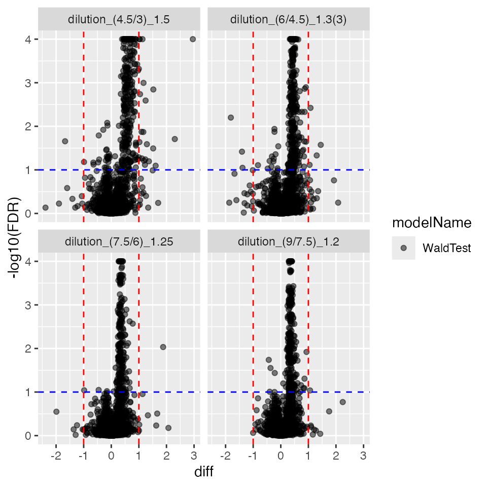
pl$histogram()$p.value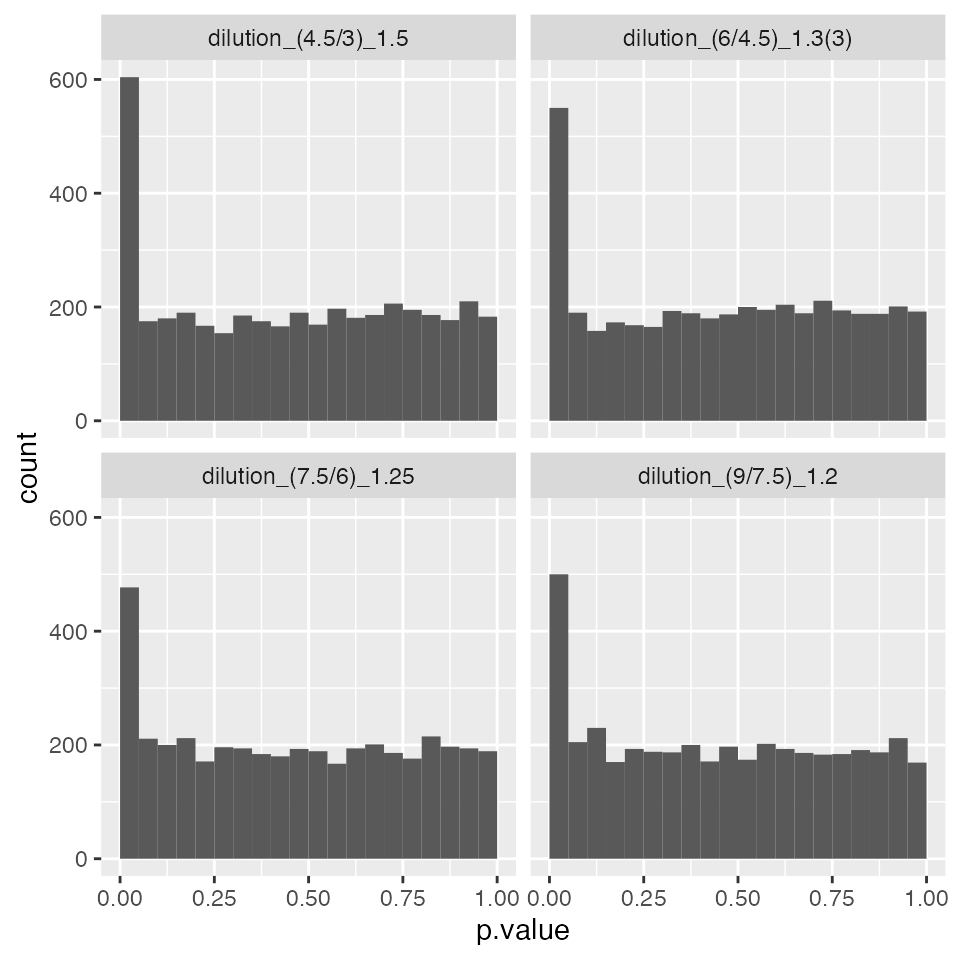
allContrasts$Prot <- contrProt$get_contrasts()

ttd <- prolfqua::ionstar_bench_preprocess(contrProt$get_contrasts())

benchmark_Prot <- prolfqua::make_benchmark(
    ttd$data,
    model_description = "med. polish and lm",
    model_name = "prolfqua_lm"
)

prolfqua::table_facade(benchmark_Prot$smc$summary, caption = "Nr of proteins with Nr of not estimated contrasts.", digits = 1)| nr_missing | protein_Id |
|---|---|
| 0 | 4042 |
| 1 | 61 |
| 2 | 39 |
| 3 | 10 |
| 4 | 13 |
#benchmark_Prot$plot_score_distribution()
benchmark_Prot$plot_FDRvsFDP()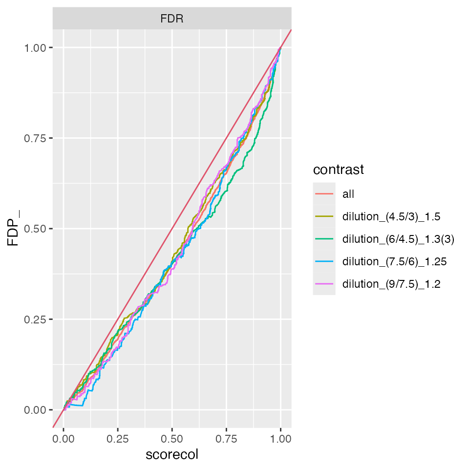
allBenchmarks$benchmark_Prot <- benchmark_ProtAdding DEqMS Moderation
DEqMS applies count-dependent variance shrinkage: proteins quantified from many peptides get less shrinkage, proteins from few peptides get more.
count_df <- lfqNormSubset$data |>
  dplyr::select(protein_Id, peptide_Id) |>
  dplyr::distinct() |>
  dplyr::count(protein_Id, name = "nr_peptides")
contrProtDEqMS <- prolfqua::ContrastsModeratedDEqMS$new(
  contrProt,
  count_df = count_df,
  count_column = "nr_peptides"
)
contrProtDEqMS$get_Plotter()$volcano()$FDR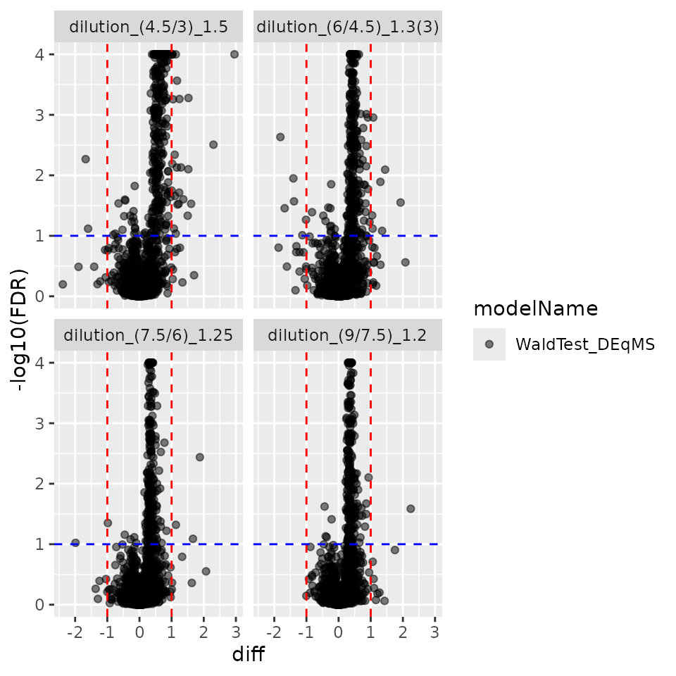
allContrasts$ProtDEqMS <- contrProtDEqMS$get_contrasts()
ttd <- prolfqua::ionstar_bench_preprocess(contrProtDEqMS$get_contrasts())
benchmark_ProtDEqMS <- prolfqua::make_benchmark(
    ttd$data,
    model_description = "med. polish and lm DEqMS moderated",
    model_name = "prolfqua_lm_DEqMS")

prolfqua::table_facade(
  benchmark_ProtDEqMS$smc$summary,
  caption = "Nr of proteins with Nr of not estimated contrasts.",
digits = 1)| nr_missing | protein_Id |
|---|---|
| 0 | 4042 |
| 1 | 61 |
| 2 | 39 |
| 3 | 10 |
| 4 | 13 |
benchmark_ProtDEqMS$plot_FDRvsFDP()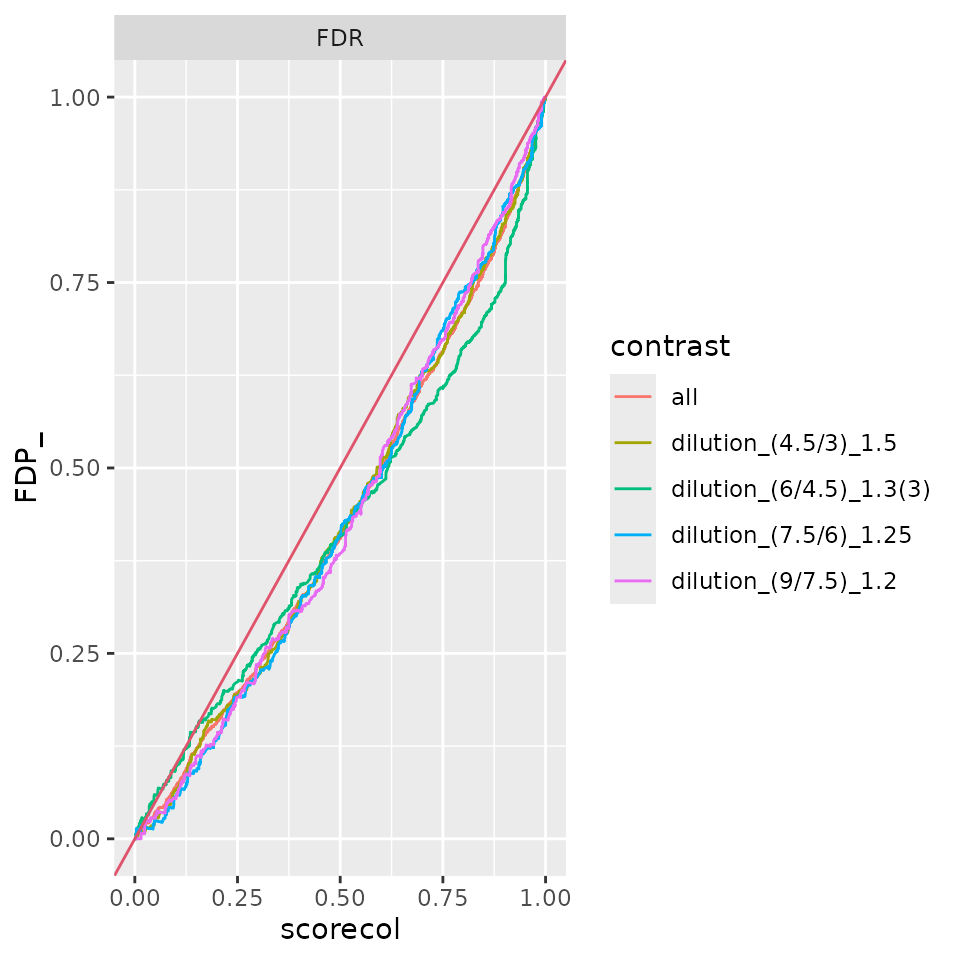
allBenchmarks$benchmark_ProtDEqMS <- benchmark_ProtDEqMSContrasts from mixed effect models
contrProtMixed <- prolfqua::Contrasts$new(modMixedProtLevel, relevantContrasts, modelName = "WaldTestMixed")

pl <- contrProtMixed$get_Plotter()
pl$volcano()$FDR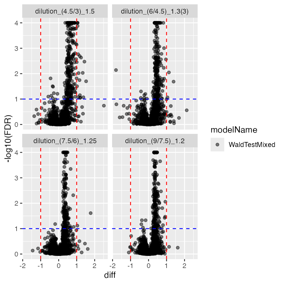
pl$histogram()$p.value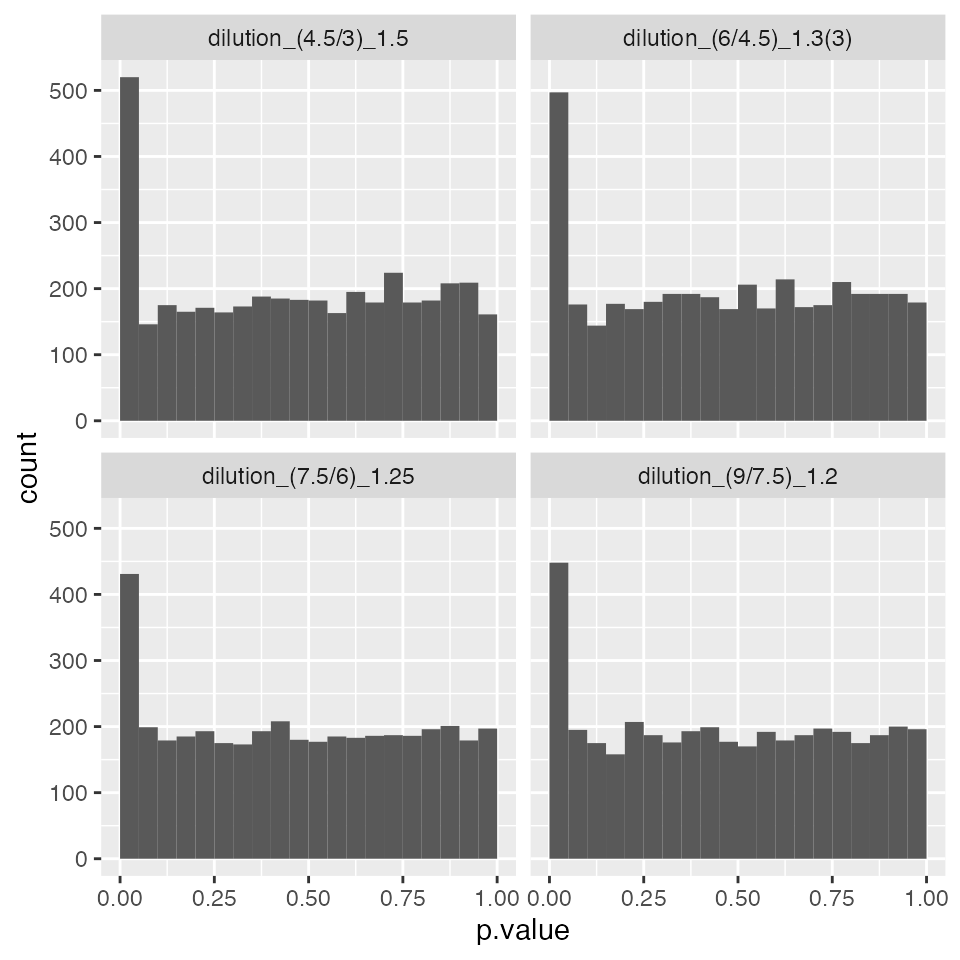
## [1] 4001
allContrasts$contrProtMixed <- contrProtMixed$get_contrasts()
ttd <- prolfqua::ionstar_bench_preprocess(contrProtMixed$get_contrasts())
benchmark_mixed <- prolfqua::make_benchmark(
    ttd$data,
    model_description = "mixed effect model",
    model_name = "prolfqua_mix_eff"
)
benchmark_mixed$complete(FALSE)
prolfqua::table_facade(benchmark_mixed$smc$summary,
caption = "Nr of proteins with Nr of not estimated contrasts.", digits = 1)| nr_missing | protein_Id |
|---|---|
| 0 | 3939 |
| 1 | 42 |
| 2 | 18 |
| 3 | 2 |
#benchmark_mixed$plot_score_distribution()
benchmark_mixed$plot_FDRvsFDP()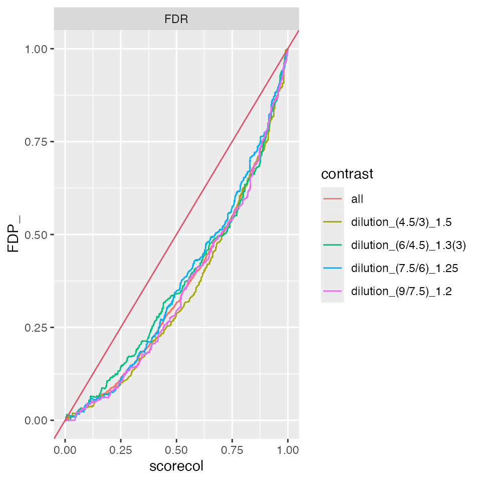
allBenchmarks$benchmark_mixed <- benchmark_mixedAdding Moderation
Since moderation requires a degrees of freedom estimate to determine the prior degrees of freedom we examine the denominator degrees of freedom produced by the methods implemented in lmerTest (see Histogram).
ctr <- contrProtMixed$get_contrasts()
df <- ctr$df
df[df > 59] <- 60
range(df)
## [1] 0.9968624 60.0000000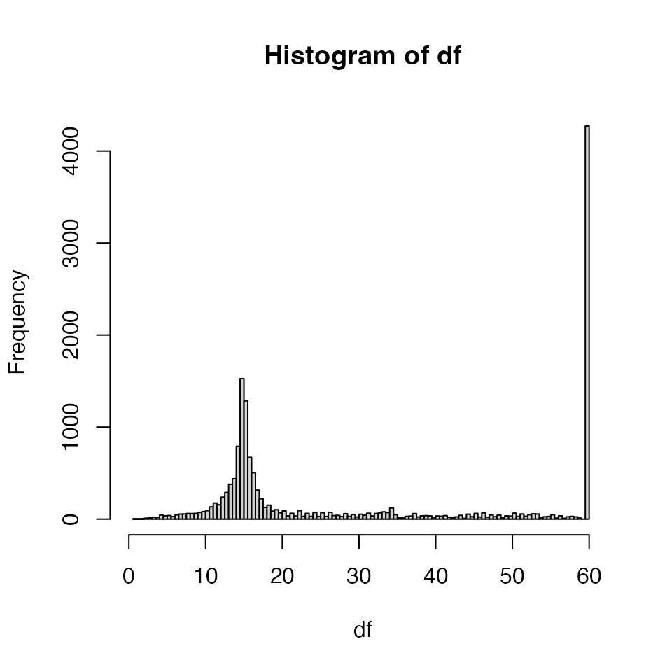
Histogram of degrees of freedom for mixed model
contrProtMixedModerated <- prolfqua::ContrastsModerated$new(contrProtMixed)
contrProtMixedModerated$get_Plotter()$volcano()$FDR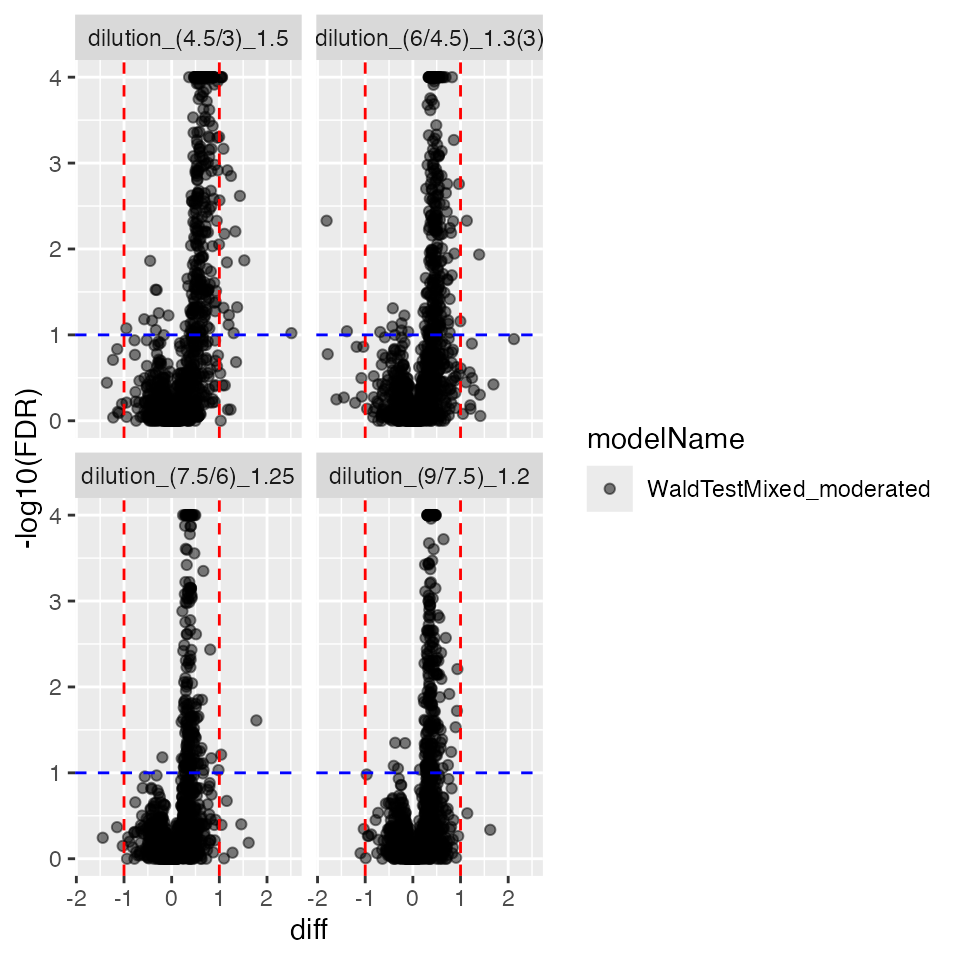
allContrasts$contrProtMixedModerated <- contrProtMixedModerated$get_contrasts()

ttd <- prolfqua::ionstar_bench_preprocess(contrProtMixedModerated$get_contrasts())

benchmark_mixedModerated <- prolfqua::make_benchmark(
    ttd$data,
    model_description = "mixed effect model moderated",
    model_name = "prolfqua_mix_eff_mod")
prolfqua::table_facade(benchmark_mixedModerated$smc$summary, caption = "Nr of proteins with Nr of computed contrasts.", digits=1)| nr_missing | protein_Id |
|---|---|
| 0 | 3939 |
| 1 | 42 |
| 2 | 18 |
| 3 | 2 |
#benchmark_mixedModerated$plot_score_distribution()
benchmark_mixedModerated$plot_FDRvsFDP()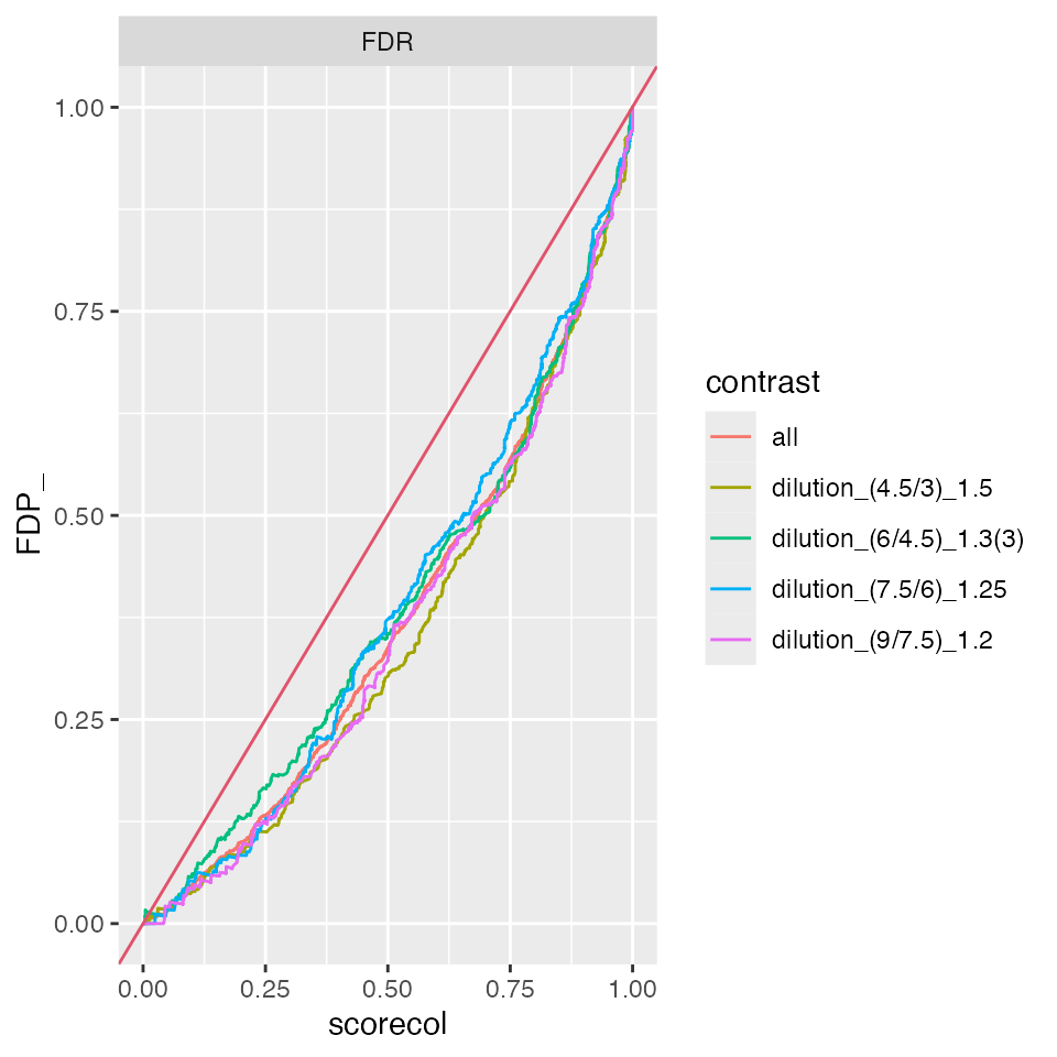
allBenchmarks$benchmark_mixedModerated <- benchmark_mixedModeratedProtein level contrasts from peptide models
To estimate regulation probabilities using the ROPECA approach we can chain the contrast computation methods. First we compute contrasts on peptide level, than we moderated the variance, t-statistics and p-values and finally we aggregate the fold change estimates and p-values.
contrastPep <- prolfqua::Contrasts$new(modLMPepLevel, relevantContrasts)
contrROPECA <- prolfqua::ContrastsModerated$new( contrastPep )  |>  prolfqua::ContrastsROPECA$new()
contrROPECA$get_Plotter()$volcano()$FDR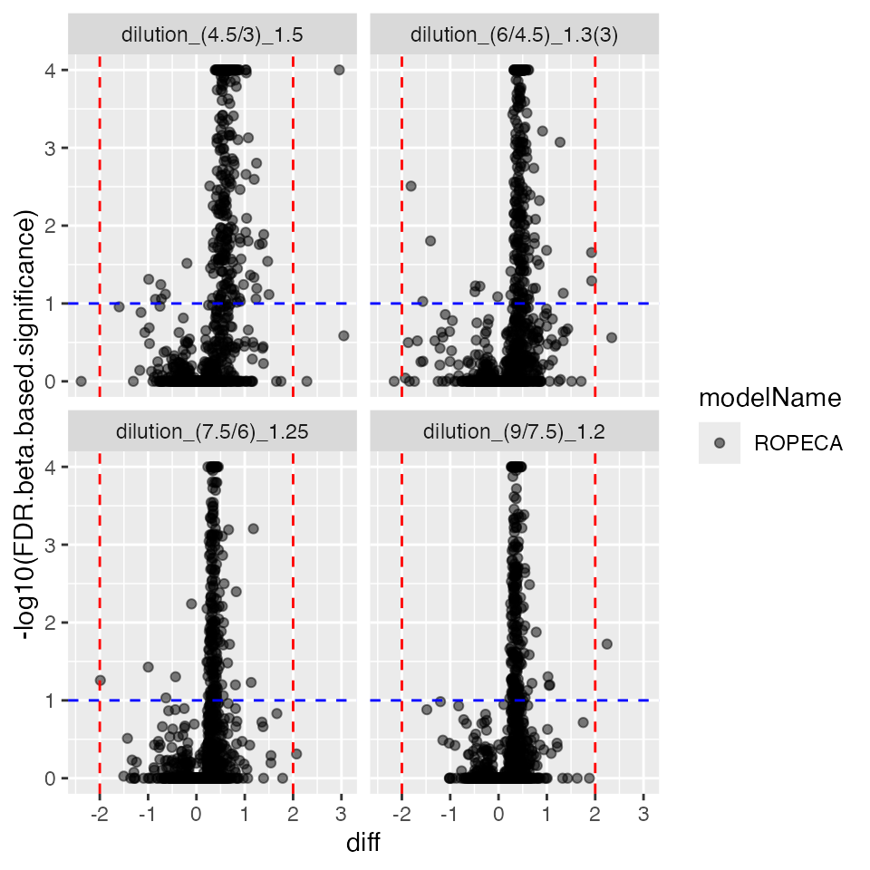
contrROPECA$get_Plotter()$histogram()$FDR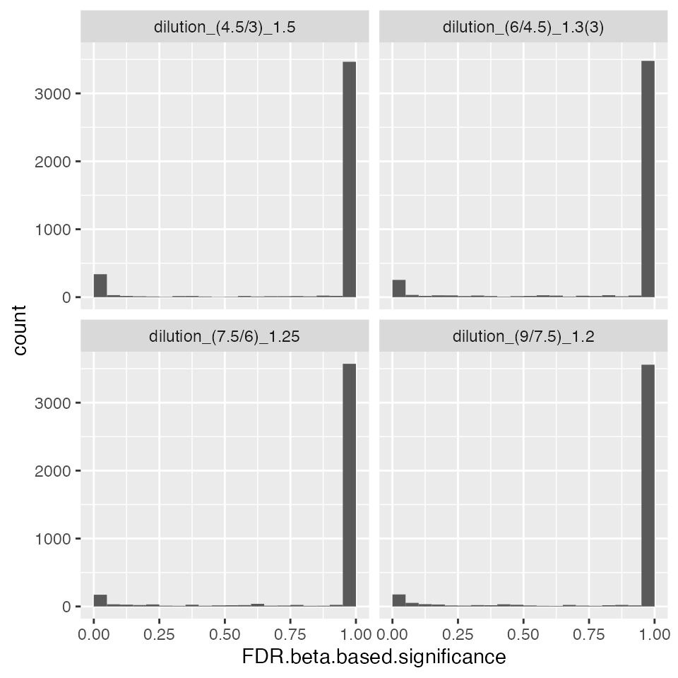
cr <- contrROPECA$get_contrasts()
ttd <- prolfqua::ionstar_bench_preprocess(cr)
benchmark_ropeca <- prolfqua::make_benchmark(
    ttd$data,
    toscale = c("beta.based.significance"),
    benchmark = list(
        list(score = "diff", desc = TRUE),
        list(score = "statistic", desc = TRUE),
        list(score = "scaled.beta.based.significance", desc = TRUE)
    ),
    model_description = "Ropeca",
    model_name = "prolfqua_ropeca",
    FDRvsFDP = list(list(score = "FDR.beta.based.significance", desc = FALSE))
)

prolfqua::table_facade(
    benchmark_ropeca$smc$summary,
    caption = "Nr of proteins with Nr of not estimated contrasts.",
digits = 1)| nr_missing | protein_Id |
|---|---|
| 0 | 4018 |
| 1 | 64 |
| 2 | 43 |
| 3 | 21 |
| 4 | 18 |
benchmark_ropeca$plot_ROC(1)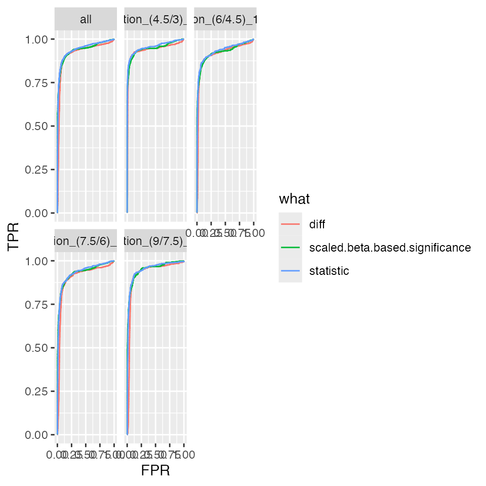
benchmark_ropeca$plot_FDRvsFDP()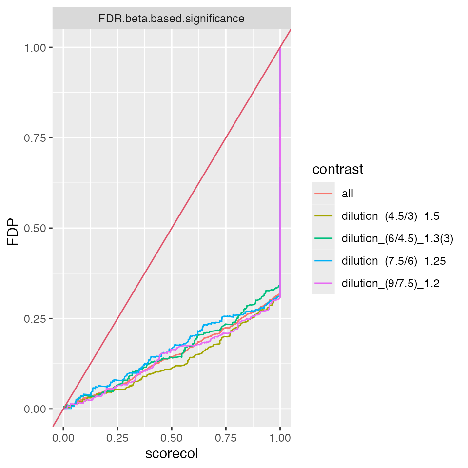
allBenchmarks$benchmark_ropeca <- benchmark_ropeca
bb <- benchmark_ropeca$pAUC_summaries()
bb$barp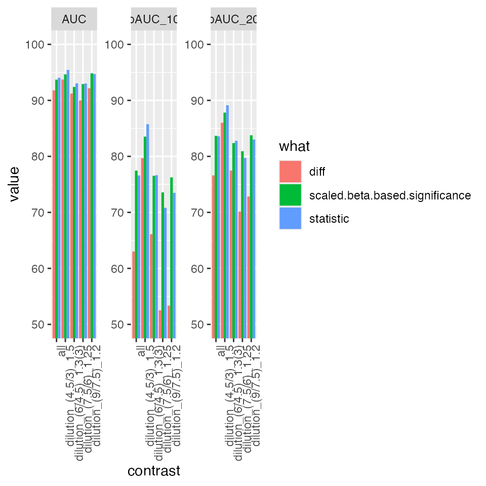
Summary of partial area under the ROC curve.
prolfqua::table_facade(bb$ftable$content, caption = bb$ftable$caption, digits = 1)| contrast | what | AUC | pAUC_10 | pAUC_20 |
|---|---|---|---|---|
| all | diff | 91.8 | 63.0 | 76.6 |
| all | scaled.beta.based.significance | 93.7 | 77.5 | 83.7 |
| all | statistic | 94.0 | 76.6 | 83.6 |
| dilution_(4.5/3)_1.5 | diff | 93.7 | 79.7 | 86.0 |
| dilution_(4.5/3)_1.5 | scaled.beta.based.significance | 94.6 | 83.5 | 87.8 |
| dilution_(4.5/3)_1.5 | statistic | 95.4 | 85.7 | 89.1 |
| dilution_(6/4.5)_1.3(3) | diff | 91.2 | 66.1 | 77.5 |
| dilution_(6/4.5)_1.3(3) | scaled.beta.based.significance | 92.4 | 76.5 | 82.4 |
| dilution_(6/4.5)_1.3(3) | statistic | 93.0 | 76.6 | 82.8 |
| dilution_(7.5/6)_1.25 | diff | 90.0 | 52.5 | 70.1 |
| dilution_(7.5/6)_1.25 | scaled.beta.based.significance | 92.9 | 73.6 | 80.9 |
| dilution_(7.5/6)_1.25 | statistic | 93.0 | 70.8 | 79.7 |
| dilution_(9/7.5)_1.2 | diff | 92.2 | 53.4 | 72.8 |
| dilution_(9/7.5)_1.2 | scaled.beta.based.significance | 94.8 | 76.3 | 83.8 |
| dilution_(9/7.5)_1.2 | statistic | 94.7 | 73.5 | 83.0 |
Contrasts from limma model
Limma uses a matrix-based linear model with empirical Bayes variance
moderation via lmFit + eBayes. This is an
alternative to the per-protein lm +
squeezeVarRob pipeline.
limma_formula <- paste0(protLFQ$config$table$get_response(), " ~ dilution.")
limma_strategy <- prolfqua::strategy_limma(limma_formula)
modLimma <- prolfqua::build_model_limma(protLFQ, limma_strategy)
modLimma$anova_histogram()$plot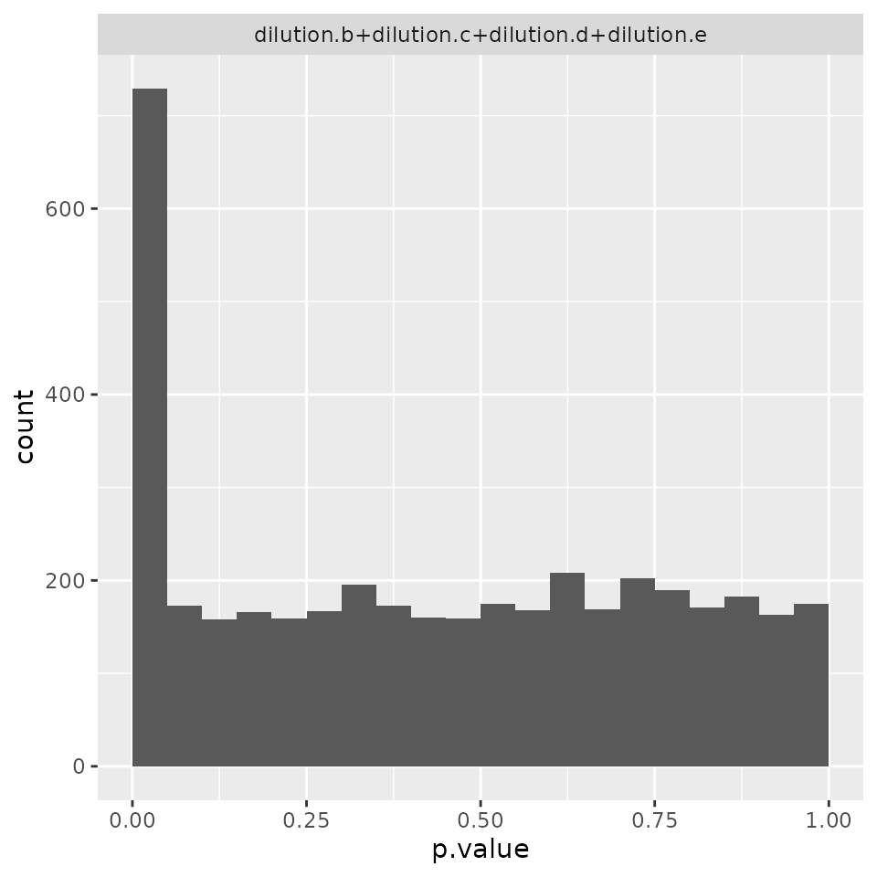
contrLimma <- prolfqua::ContrastsLimma$new(modLimma, relevantContrasts)
contrLimma$get_Plotter()$volcano()$FDR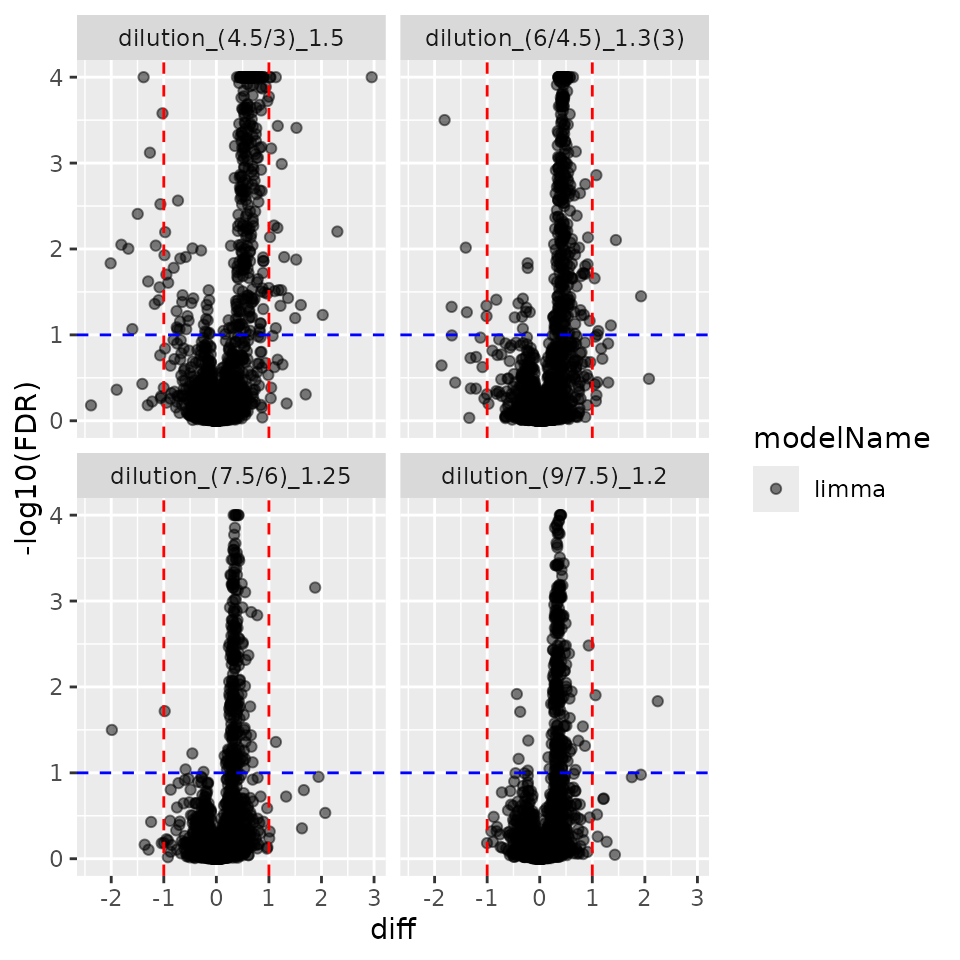
allContrasts$Limma <- contrLimma$get_contrasts()
ttd <- prolfqua::ionstar_bench_preprocess(contrLimma$get_contrasts())
benchmark_Limma <- prolfqua::make_benchmark(
    ttd$data,
    model_description = "med. polish and limma",
    model_name = "prolfqua_limma")

prolfqua::table_facade(
  benchmark_Limma$smc$summary,
  caption = "Nr of proteins with Nr of not estimated contrasts.",
digits = 1)| nr_missing | protein_Id |
|---|---|
| 0 | 4043 |
| 1 | 64 |
| 2 | 34 |
| 3 | 23 |
| 4 | 14 |
benchmark_Limma$plot_FDRvsFDP()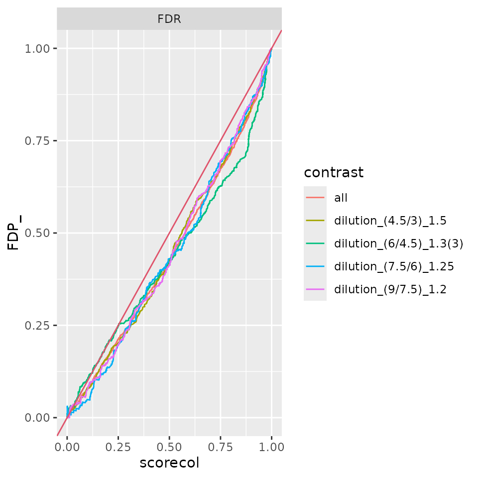
allBenchmarks$benchmark_Limma <- benchmark_LimmaMerging contrasts of two models.
Here we merge contrasts estimates from linear models and from the
models with imputation using merge_contrasts_results. We
prefer the contrasts estimated with linear models and if missing augment
them with the contrasts estimated with imputation.
all <- prolfqua::merge_contrasts_results(prefer = contrProt, add = contrImp)

merged <- prolfqua::ContrastsModerated$new(all$merged)
ttd <- prolfqua::ionstar_bench_preprocess(merged$get_contrasts())
benchmark_merged <- prolfqua::make_benchmark(
    ttd$data,
    model_description = "merge of prot moderated and imputed",
    model_name = "prolfqua_merged")

prolfqua::table_facade(
  benchmark_merged$smc$summary,
  caption = "Nr of proteins with Nr of not estimated contrasts.",
digits = 1)| nr_missing | protein_Id |
|---|---|
| 0 | 4178 |
#benchmark_mixedModerated$plot_score_distribution()

benchmark_merged$plot_FDRvsFDP()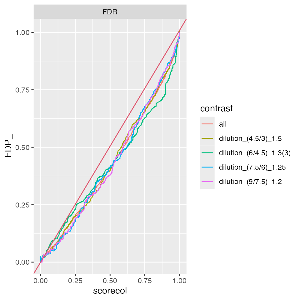
benchmark_merged$plot_ROC(xlim = 0.15)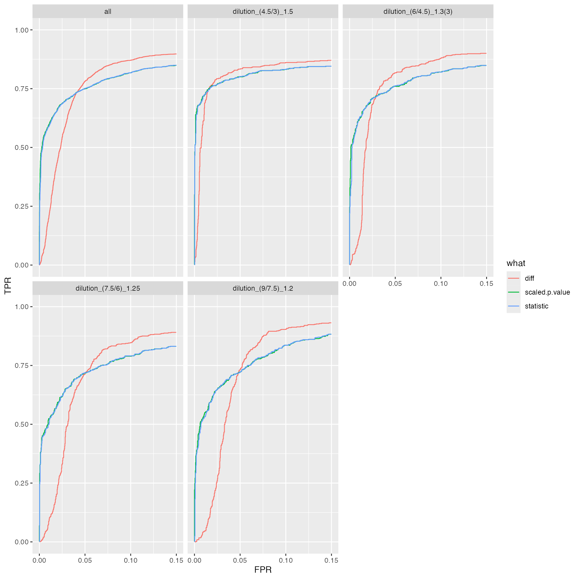
ROC curves for merged benchmark
bb <- benchmark_merged$pAUC_summaries()
bb$barp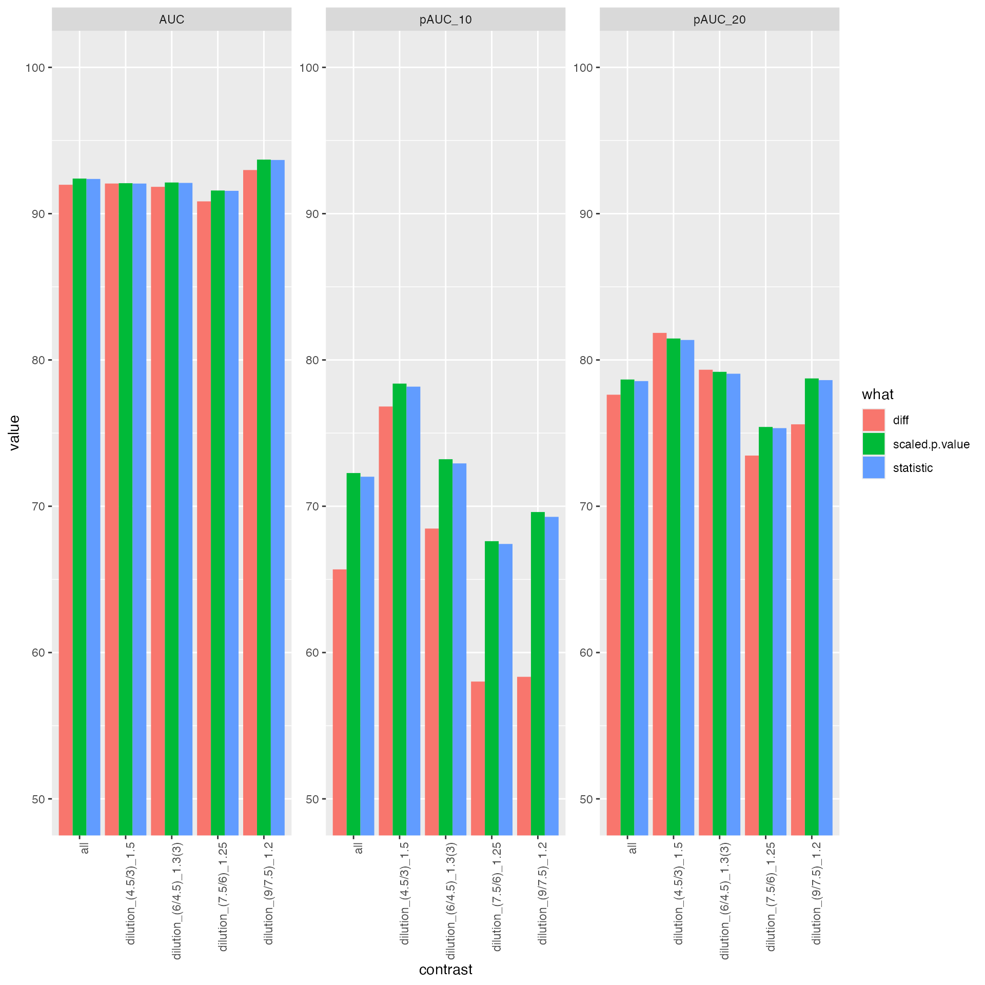
ROC curves for merged benchmark
tmp <- prolfqua::table_facade(bb$ftable$content, caption = bb$ftable$caption, digits=1)
knitr::kable((bb$ftable$content))| contrast | what | AUC | pAUC_10 | pAUC_20 |
|---|---|---|---|---|
| all | diff | 91.97551 | 65.68438 | 77.62483 |
| all | scaled.p.value | 92.39791 | 72.27018 | 78.66324 |
| all | statistic | 92.37255 | 72.01880 | 78.55498 |
| dilution_(4.5/3)_1.5 | diff | 92.05969 | 76.81841 | 81.84991 |
| dilution_(4.5/3)_1.5 | scaled.p.value | 92.08219 | 78.38420 | 81.46662 |
| dilution_(4.5/3)_1.5 | statistic | 92.05802 | 78.17602 | 81.36627 |
| dilution_(6/4.5)_1.3(3) | diff | 91.83409 | 68.47558 | 79.33140 |
| dilution_(6/4.5)_1.3(3) | scaled.p.value | 92.12960 | 73.21443 | 79.18805 |
| dilution_(6/4.5)_1.3(3) | statistic | 92.10155 | 72.92950 | 79.05838 |
| dilution_(7.5/6)_1.25 | diff | 90.84027 | 58.01783 | 73.46430 |
| dilution_(7.5/6)_1.25 | scaled.p.value | 91.58246 | 67.61285 | 75.42066 |
| dilution_(7.5/6)_1.25 | statistic | 91.55992 | 67.42319 | 75.33994 |
| dilution_(9/7.5)_1.2 | diff | 92.98192 | 58.34157 | 75.60017 |
| dilution_(9/7.5)_1.2 | scaled.p.value | 93.69456 | 69.60472 | 78.73728 |
| dilution_(9/7.5)_1.2 | statistic | 93.66876 | 69.27524 | 78.62260 |
allBenchmarks$benchmark_merged <- benchmark_mergedMerged with DEqMS moderation
merged_deqms <- prolfqua::ContrastsModeratedDEqMS$new(
  all$merged,
  count_df = count_df,
  count_column = "nr_peptides"
)
ttd <- prolfqua::ionstar_bench_preprocess(merged_deqms$get_contrasts())
benchmark_merged_deqms <- prolfqua::make_benchmark(
    ttd$data,
    model_description = "merge of prot DEqMS moderated and imputed",
    model_name = "prolfqua_merged_DEqMS")

benchmark_merged_deqms$plot_FDRvsFDP()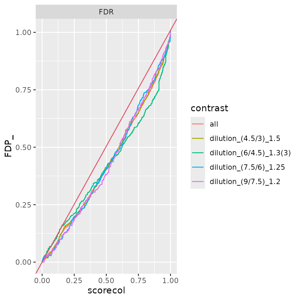
allBenchmarks$benchmark_merged_deqms <- benchmark_merged_deqmsMerged with limma
all_limma <- prolfqua::merge_contrasts_results(prefer = contrLimma, add = contrImp)
merged_limma <- prolfqua::ContrastsModerated$new(all_limma$merged)
ttd <- prolfqua::ionstar_bench_preprocess(merged_limma$get_contrasts())
benchmark_merged_limma <- prolfqua::make_benchmark(
    ttd$data,
    model_description = "merge of limma and imputed",
    model_name = "prolfqua_limma_merged")

benchmark_merged_limma$plot_FDRvsFDP()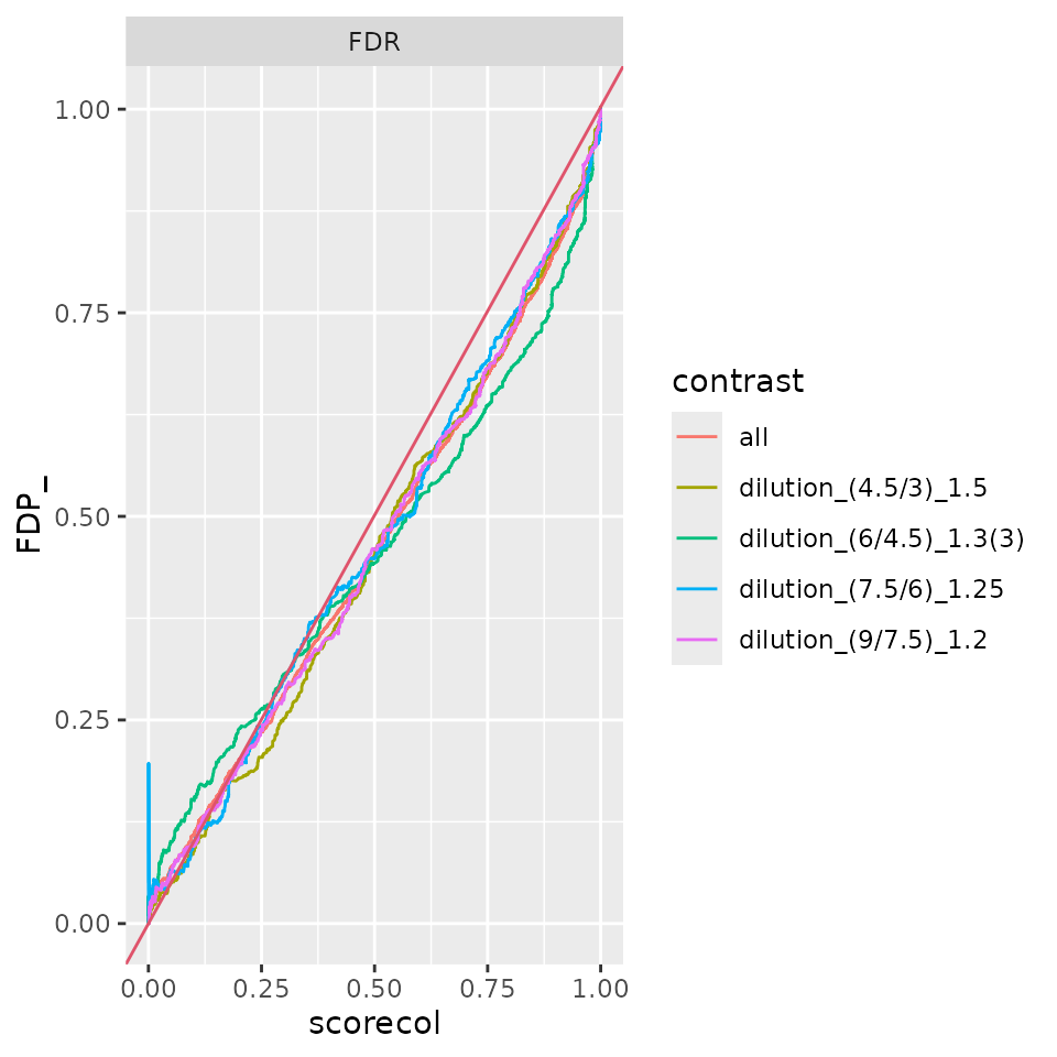
allBenchmarks$benchmark_merged_limma <- benchmark_merged_limma
same <- all$same
allBenchmarks$benchmark_Prot$smc$summary

ttd <- prolfqua::ionstar_bench_preprocess(same$get_contrasts())
benchmark_same <- prolfqua::make_benchmark(
    ttd$data,
    model_description = "imputed_same_as_lm",
    model_name = "imputed_same_as_lm")

prolfqua::table_facade(benchmark_same$smc$summary, caption = "Nr of proteins with Nr of not estimated contrasts.", digits=1)
benchmark_same$plot_FDRvsFDP()
benchmark_same$plot_ROC(xlim = 0.15)
bb <- benchmark_same$pAUC_summaries()
bb$barp

prolfqua::table_facade(bb$ftable$content, caption = bb$ftable$caption, digits=1)

allBenchmarks$benchmark_same <- benchmark_same
Comparing various models
The table below summarizes the contrast estimates produced which will be benchmarked.
| Model | Contrast | Moderation | Aggregation | |
|---|---|---|---|---|
| Protein abundance | lm | o | o | |
| Protein abundance | lm | o | o (DEqMS) | |
| Protein abundance | limma | o | o (eBayes) | |
| Protein abundance Imputed | pooled variance | o | o | |
| Peptide abundance | lmer | o | o | |
| Peptide abundance | lm | o |
ttt <- sapply(allBenchmarks, function(x){x$complete(FALSE)})
res <- purrr::map_df(allBenchmarks, function(x){x$pAUC()})
resAllB <- res |> dplyr::filter(contrast == "all")

bb <- resAllB |> dplyr::mutate(whatfix = dplyr::case_when(what == "scaled.beta.based.significance" ~ "scaled.p.value", TRUE ~ what))

ggplot2::ggplot(bb, ggplot2::aes(x = Name, y = pAUC_10)) +
  ggplot2::geom_bar(stat = "identity") +
  ggplot2::facet_wrap(~whatfix)  +
  ggplot2::coord_cartesian(ylim = c(min(bb$pAUC_10),max(bb$pAUC_10))) +
  ggplot2::theme_minimal() +
  ggplot2::theme(axis.text.x = ggplot2::element_text(angle = -90, vjust = 0.5))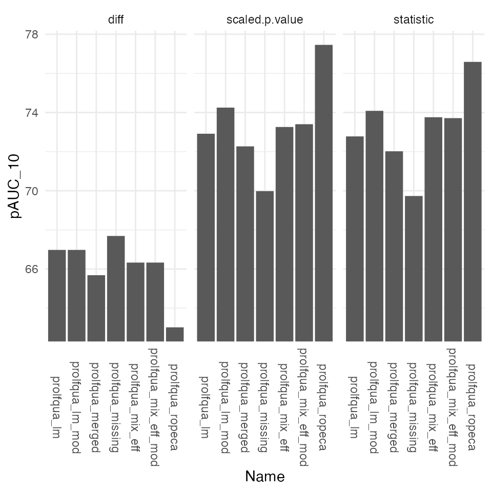
Partial area under the ROC curve at 10% FPR.
ggplot2::ggplot(bb, ggplot2::aes(x = Name, y = pAUC_20)) +
  ggplot2::geom_bar(stat = "identity") +
  ggplot2::facet_wrap(~whatfix)  +
  ggplot2::coord_cartesian(ylim = c(min(bb$pAUC_20),max(bb$pAUC_20))) +
  ggplot2::theme_minimal() +
ggplot2::theme(axis.text.x = ggplot2::element_text(angle = -90, vjust = 0.5)) 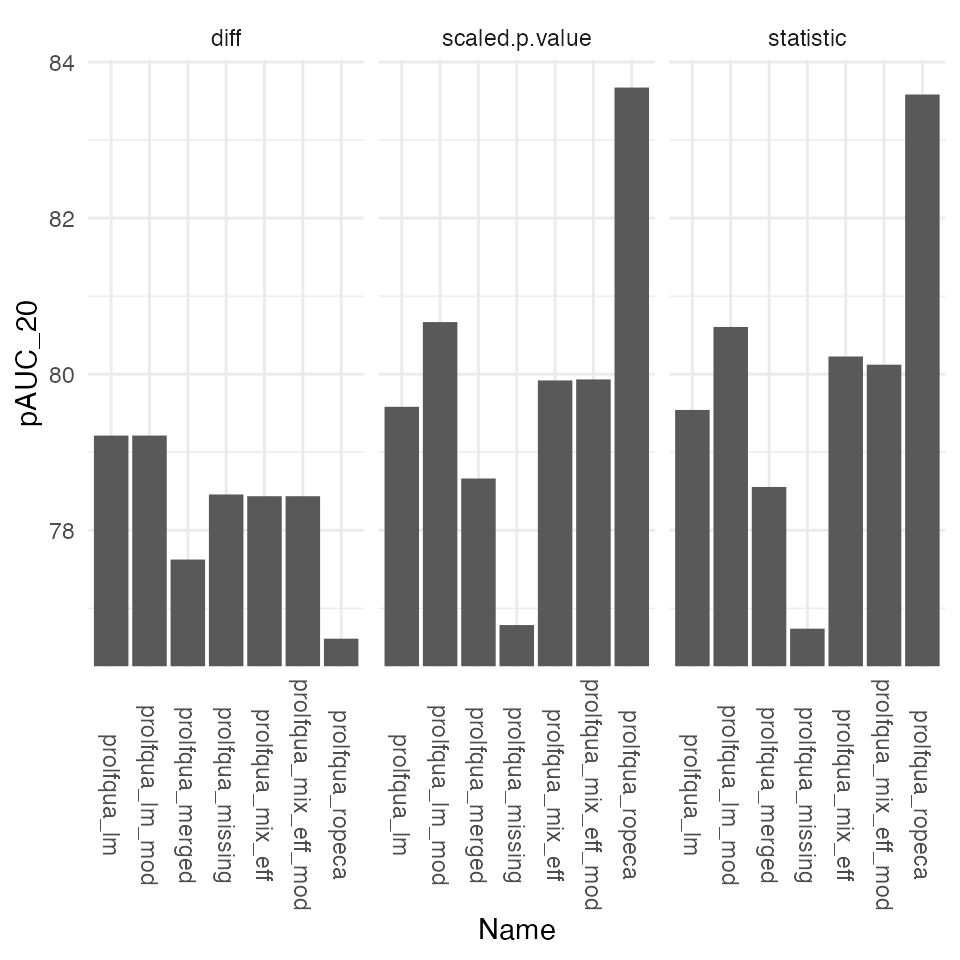
Look at the nr of estimated contrasts.
dd <- purrr::map_df(allBenchmarks, function(x){res <- x$smc$summary; res$name <- x$model_name;res})


dd <- dd |> dplyr::mutate(nrcontrasts = protein_Id * (4 - as.integer(nr_missing)))
dds <- dd |> dplyr::group_by(name) |> dplyr::summarize(nrcontrasts = sum(nrcontrasts))

dds |> ggplot2::ggplot(ggplot2::aes(x = name, y = (nrcontrasts - min(nrcontrasts)))) +
  ggplot2::geom_bar(stat = "identity") +
  ggplot2::theme(axis.text.x = ggplot2::element_text(angle = -90, vjust = 0.5)) +
  ggplot2::geom_text(ggplot2::aes(label= nrcontrasts), position = ggplot2::position_dodge(width=0.9), vjust=-0.25)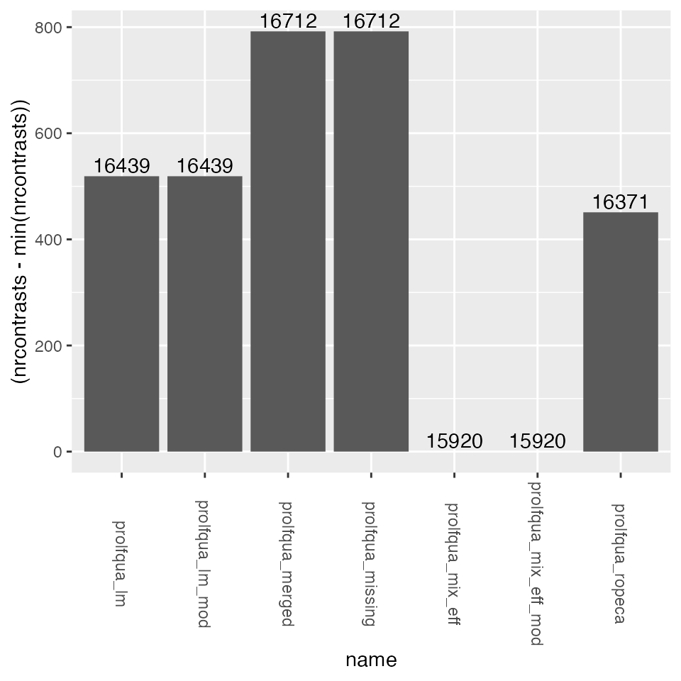
NR of estimated contrasts
Plot FDR vs FDP
dd <- purrr::map_df(allBenchmarks, function(x){res <- x$get_confusion_FDRvsFDP(); res$name <- x$model_name;res})

dd |> ggplot2::ggplot(ggplot2::aes(y = FDP_,  x  = scorecol )) +
  ggplot2::geom_line(ggplot2::aes(color = model_name)) +
  ggplot2::facet_wrap(~contrast) +
  ggplot2::geom_abline(intercept = 0, slope = 1, color = 2)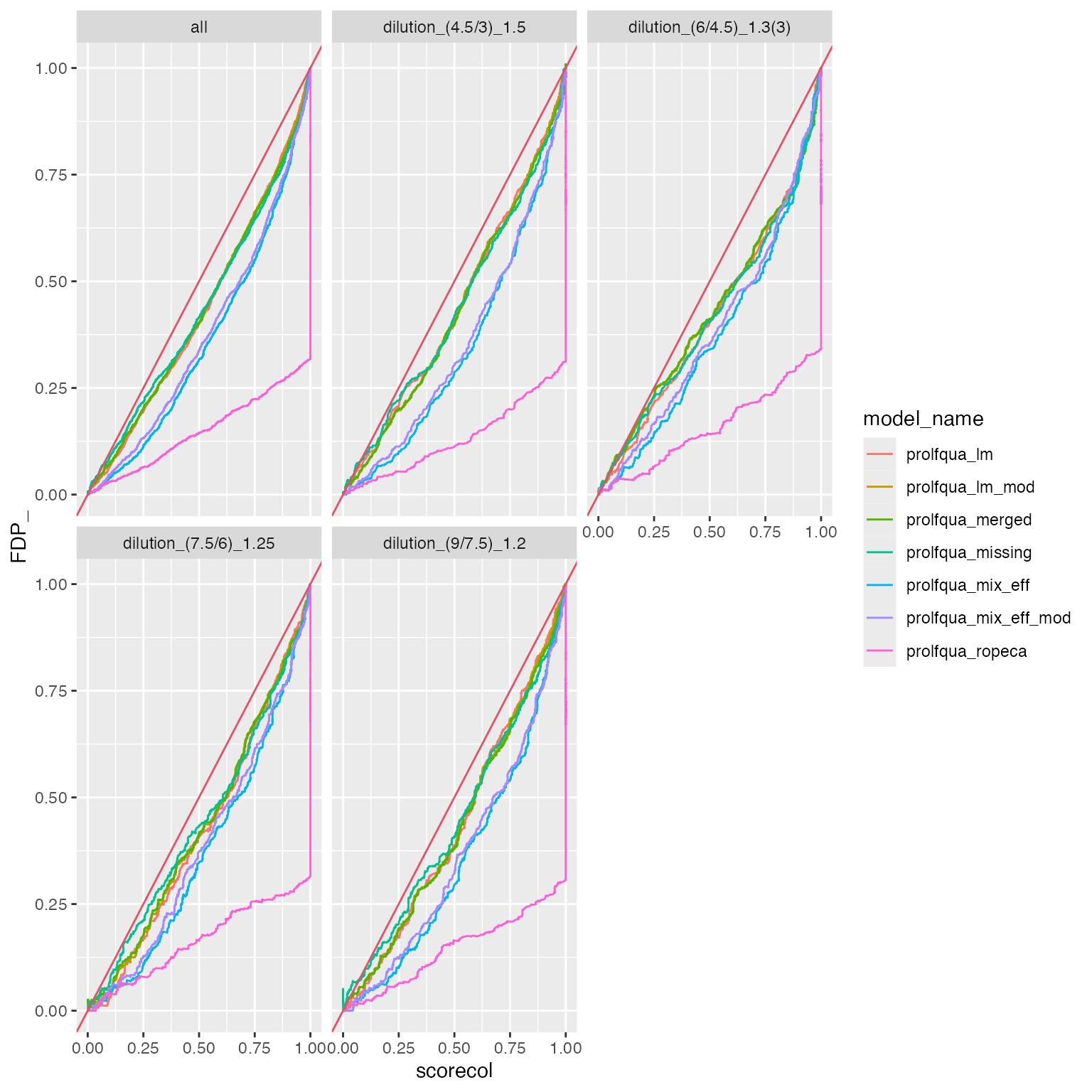
Compare FDR estimate with false discovery proportion (FDP).